10: Responsibility Accounting

Chapter 10 Guided Practice Problems

10.1 Decentralized Decision Rights

10.1.1 Small Firms vs. Large Firms

In a small firm the owner possesses most of the knowledge and exercises most of the decision rights. If a customer is upset, the owner is likely involved in the decision of whether to offer a refund, sometimes making the decision himself or herself. If there are multiple vendors to choose from, the owner is likely involved in the vendor decision, sometimes making that decision too.

As the firm grows larger, it becomes less and less practical for the owner to be closely involved in these decisions. The owner will be less informed of ground-level facts to base the decision on and will have a higher and higher marginal cost for his or her time.

In the same way that knowledge is decentralized in large firms, decision rights in larger firms are also delegated and decentralized. Someone other than the owner needs to make customer refund decisions or vendor decisions in most cases.

But what if the subordinate who is delegated authority doesn’t do what’s good for the firm? Managers might make a choice that’s good for them personally but bad for other downstream components of the firm. (Like in Chapter 9 I’m approaching this topic as a rebuttal to the assumption I made at the beginning of the textbook that managers always seek to maximize firm profit.)

Many firms use responsibility accounting as the solution to this problem.

Responsibility accounting is accounting information used to hold managers accountable for the decision rights delegated to them.

I’ve been biting off bits and pieces around this topic since Chapter 2. Determining product cost, as discussed in Chapters 4 through 6, is important for holding managers responsible for their costs. Variance analysis, covered in Chapter 7, is a form of responsibility accounting.

This chapter addresses the topic head-on with a few key responsibility accounting tools.

10.1.2 Responsibility Centers

Responsibility accounting focuses on decision rights delegated to middle-level managers. These aren’t the only decision rights delegated within large firms, but they are often the focus of responsibility accounting tools, and they are a good illustration of the general idea. I will focus on middle managers too.

Middle managers include division managers, department managers, regional managers, and general/branch managers. They oversee a significant sub-unit of the firm and are supposed to execute the firm’s strategy within that sub-unit of the firm.

Middle managers’ decision rights depends can be split into three types, based on two key questions.

1. Does this manager control revenue?
2. Does this manager control costs?

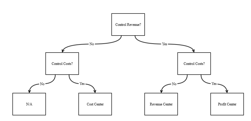
Cost center managers run departments such as accounting, information technology, purchasing, human resources, maintenance, quality assurance, and research and development. Often factory production and operation are managed as a cost center. Revenue center managers typically oversee a sales office or a storefront. A profit center manager is over both costs and revenue, such as a factory manager, branch manager, or regional manager.

(Materiality and directness are important in answering these questions. A cost center manager might control some small revenue stream and a revenue center manager might control some small costs related to the sales team. This does not make transform these two into profit centers managers, per se. Likewise having an indirect influence on costs or revenues often isn’t enough to justify to change a manager’s responsibility center.)

These three types of responsibility centers are named after their income statement effects: revenue, cost, and profit (I add a fourth type in Section 10.4 which does not follow this pattern). Responsibility accounting for these responsibility centers is usually based on the income statement accounting information the manager controls.

That is, if a department manager can affect the firm’s costs, he or she should be held accountable for his or her effect on firm cost. If a sales manager can affect the firm’s revenue, he or she should be held accountable for his or her effect on firm revenue. If a branch manager can affect both cost and revenue, he or she should be held accountable for his or her effect on firm profit.

The problem is that cost centers, revenue centers, and profit centers do not exist in isolation. They almost always interact and depend on each other. A factory that’s considered a profit center might depend on cost centers like the accounting, information technology, human resources, and research and development departments. It might depend on a separate sales team, a revenue center. It might produce an intermediate good that is shipped to the next factory in the chain, another profit center

Section 10.2 and Section 10.3 cover two common methods of trying to account for this and sort out responsibility across interdependent departments within the firm.

10.2 Service Department Cost Allocations

10.2.1 Interdependency

Cost centers often provide services to support each other. Some of these cost centers are sometimes called service departments and the cost centers they provide benefits to are sometimes called production departments.

Most service department costs are incurred on behalf of the production departments they serve. Firms often allocate service department costs to production departments. The rationale for this is straightforward. Without the production department using the service department’s service, the cost of that service probably wouldn’t be incurred.

What is less straightforward is how much the allocation should be.

Firms usually have more than one service department and more than one production department. These service departments sometimes have interdependency, meaning they rely on services from other service departments.

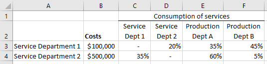
This is an example of interdependency. 20% of Service Department 1’s services are consumed by another Service Department 2, and 35% of Service Department 2’s services are consumed by another Service Department 1.

A significant portion of the $500,000 in Department 2’s costs is likely due to the work this department does for Department 1. Should all $500,000 of Department 2’s costs be allocated to the production departments?

10.2.2 Direct Method

The direct method effectively says, “Yes. We do not care about interdependency among service departments.” Each service department allocates its costs directly to production departments based on those departments’ use of the service firm’s service (usually as measured by an appropriate cost driver).

That means this method can be a student’s favorite. Still, there are ways to get this kind of calculation wrong.

Let’s look at an example of this.

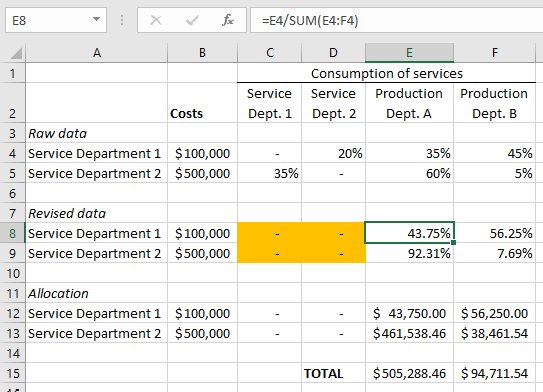
Note that this example, like all examples in Section 10.2, I already calculate percentages of cost driver consumption for you. In practice that step must be done first. I highlight the interdependent percentages among service departments to show how, under the direct method, you ignore these, treating them as if they were all 0%.

To complete the direct method, you form new percentages of service department consumption by dividing a given production department’s consumption by the total consumption by production departments only (look at the formula in cell E8). 80% of Service Department 1’s services were consumed by production departments. Of that 80%, 43.75% was consumed by Production Department A.

Production Department A receives 43.75% of Service Department 1’s $100,000 in costs. This means a cost allocation of $43,750.

Note that the method is simple but less accurate. If there is interdependency among service departments, the direct method is the least accurate of the methods covered in this chapter.

10.2.3 Step-Down Method

Using the step-down method, the firm attempts to roughly approximate the interdependency between service departments through its cost allocation process.

1. The service department that serves other service departments the most allocates its costs to production and service departments.
2. The service department that serves other service departments the second-most allocates its costs to production and service departments but not to the service department that allocated costs in the first step.
3. The service department that serves other service departments the third-most allocates its costs to production and service departments but not to the service departments that allocated costs in the first and second step.
4. Etc.

The key is to think of a stairway. Each step represents a service department. Costs allocated between service departments are like rolling a ball down the stairway. It bounces on each step below whatever step it starts on, but it can’t roll up the stairs to bounce on steps above where it started. In the same way costs from one service department are allocated to all production departments and to all service departments below them on the stairway (but to none of the service departments above them).

Here’s the same example I used to illustrate the direct method, but now I use the step-down method to allocate costs. Because Service Department 2 serves Service Department 1 more than the reverse (i.e. 35% > 20%), I place Service Department 2 at the top step in this example (i.e. that department’s costs are allocated first).

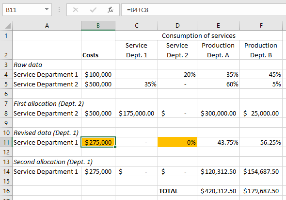
The highlighted cells are those that have to be changed after the first allocation.

The first change is that Service Department 1 acts like the service departments above it on the steps do not consume its services (Service Department 2 in this case). Service Department 1 recalculates how much of its services are consumed by production departments and any down-step service departments accordingly. (If there were a third service department, its consumption of Service Department 1’s services would be included in the denominator.)

The second change is that Service Department 1 has a higher total cost. That is because of the allocation from Service Department 2 to Service Department 1. Look at the formula for cell B11.

Notice that this method produces significantly different allocations to the two production departments. This is because almost all of that $500,000 of cost from Service Department 2 was being allocated to Production Department A under the direct method. The step-down method has more appropriately assigned some of that cost to Service Department 1, and services from Service Department 1 are more evenly consumed by the two production departments. Ultimately this leads to more of Service Department 2’s costs going to Production Department B.

You get different answers depending on the order in which the firm steps down its service departments’ costs. Not all firms order service departments using the same rationale I explained above. Step-down order can be the source of significant inter-department debate and negotiation.

All the same, if there is interdependency among service departments, the step-down method will always be more accurate than the direct method.

10.2.4 Reciprocal Method

The reciprocal method mathematically solves for interdependence between the two service departments.

It’s actually not that crazy if you set it up correctly.

The data in the example above gives you enough information to form mathematical identities to equate each service department’s costs relative to each other. Combining these identities through a system of equations solves for the exact interdependency between service departments. (It can require mathematical software to do this with more than two departments).

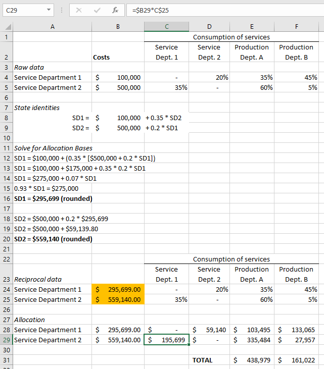
Note that the “reciprocal data” lists the cost from each department as being much higher than the raw costs from each service department. This reciprocal data includes all the service department’s costs as well as costs it has caused in other service departments (while accounting for reciprocal interdependency from that department as well). In the end the procedure for calculating the allocation is simply multiplying the reciprocal data cost number by the consumption percentage. Look at the formula for cell C29.

The reciprocal method is the most accurate allocation method.

(Of course that’s no guarantee. The reciprocal method can still be fairly inaccurate, especially if the chosen cost drivers don’t account for departments’ consumption of service department services very well. I simply mean that, assuming interdependency, the reciprocal method should always be more accurate than the other allocation methods in this chapter, ceteris paribus. If there isn’t interdependency among service departments, then all methods should be equally accurate.)

One big downside of the reciprocal method is that it is slightly more difficult to execute and understand. This is especially true if there are a multitude of service departments. Managers receiving service department costs often want an easy answer for why they are being allocated (or charged) these costs. Pointing to a complex system of equations as the answer can be very unsatisfying to them.

10.3 Transfer Pricing

10.3.1 Types of Transfer Prices

In Section 10.2 I discussed how service departments support production departments. Sometimes production departments support each other. If a production department produces a part that is used by a subsequent production department, it is often important to set up a transfer price.

Transfer prices is the price that is charged (at least in the books) by one production department for an input to another production department within the company.

Transfer prices allow the firm to better separate the performance of the selling department and the performance of the buying department. Transfer prices help each cost center or profit center manager to be held accountable for those costs he or she controls and not those costs he or she does not control.

Transfer prices can be especially important when the selling department can sell the input on an external market. Transfer prices remove at least some of the cost for internal sales (the costs are moved to the buying department by virtue of the transfer price) and the remaining costs better represent the selling department’s costs for selling its input externally.

Selling departments, obviously, would prefer a higher transfer price, because that moves more input production costs to the buying department. Buying departments prefer a lower transfer price because that keeps more of the input production costs in the selling department.

Firms set transfer prices in various ways, including the following.

1. Market price (for selling department or buying department)
2. Full absorption cost
3. Full absorption cost plus markup
4. Variable costs
5. Negotiated price

None of these is the “best” method for all firms. Each of these transfer price policies favors one department over another. Market prices and absorption cost plus markup most likely benefit the selling department because they move the most cost to the buying department. Absorption cost without markup and variable costs usually favor the buying department because they typically allow the buying department to buy the input for less than it costs on the external market.

10.3.2 Negotiated Transfer Prices

The negotiated price is the most interesting option, for my purposes at least. Negotiated prices can be influenced unduly by the managers’ personalities and social standing within the firm, but many firms see them as the best opportunity to satisfy both department managers.

A negotiated price is not determined until actual negotiations occur. But the ceiling and floor for the negotiated transfer price can be calculated beforehand.

Negotiated transfer price ceiling is the buyer’s market price. The buyer would not agree to an internal transfer price higher than what it costs them to buy the same input on the external market.

Negotiated transfer price floor is the seller’s variable costs plus their opportunity costs. They would not want to sell the product for less than it costs to make it. The equation for this looks like the equation for special order floor prices (from Chapter 3).

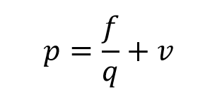
As for the variable f, there usually aren’t any additional fixed costs for selling the product internally.

(Remember, you ignore regular fixed manufacturing costs. The only fixed costs we’d be interested in are those that would have to be incurred to sell internally at all, just like in special orders covered in Chapter 3. Usually selling departments are already pre-configured to have all the knowledge, equipment, and licenses to complete the product for sale internally.)

Lost contribution margin from lost external sales is still important, though. This is usually the only fixed cost in this kind of calculation.

One additional wrinkle in these decisions: variable costs for external sales. Often the selling department can save on some sales or distribution costs by selling internally. Any variable costs that are not incurred on internal sales should not be considered a variable cost, v, that automatically goes into the price floor. The selling department will not incur those costs to sell internally. Why would the buying department be expected to pay for costs not being incurred (apart from a concession made during transfer price negotiations)?

That said, you still need these external sales-related variable costs to calculate unit contribution margin, which is required for calculating the opportunity cost. (Notice that the $25 unit contribution margin in the example above incorporates the $5 variable sales cost for external sales.)

10.4 Return on Investment and Residual Income

10.4.1 Investment Centers

Some profit center managers also have investment rights. Investment rights are decision rights to start, modify, and end capital projects and capital assets. If the manager has investment rights the manager is over an investment center.

New product lines, new buildings, new equipment, new branches, etc. are all examples of projects or assets that managers in an investment center could control.

The income statement-based responsibility accounting that works for managers of cost centers, revenue centers, and profit centers is insufficient for holding investment center managers responsible for their investment rights. Income statement numbers are relatively short-term (i.e. annual) compared to the long-term capital projects and assets that are affected by these investment rights.

The firm needs additional metrics for investment rights.

The two I will cover are (1) return on investment and (2) residual income. Return on investment is the profit from the capital project or asset divided by the investment for that capital projector asset. Residual Income is the income earned above and beyond the cost of capital.

10.4.2 Return on Investment (ROI)

Return on investment is one of several similar notions such as return on equity, return on debt, return on assets, etc. In each case the firm has made some financial move and wants to know the effect of that move on firm profit. How much does that move return to the firm?

In this case the manager has rights over the investments in his or her department of the firm and incentives can be tied to the return on these investments. Then the firm cares about the managers’ overall return on investment (i.e. incentives tied to the overall investment, or assets, of the manager’s department), and the manager evaluates current and new projects on a per-project basis (i.e. the manager evaluates individual projects’ return on investment).

Because return on investment is a figure that’s intended for long-term investments, future-year dollar amounts should be discounted back to present value.

One of the great benefits of return on investment is that it is expressed as a percentage (in decimal form). Or cents of profit per dollar invested. This makes it imminently comparable across projects, departments, companies, and industries of different sizes and types. Having a common definition of return on investment helps the figure be immediately understood.

The problem with return on investment is that it can lead managers’ interests to diverge from the interests of the firm. If a manager has a relatively high return on investment now, he or she is likely to turn down investments that are below this return on investment. Initiating those investments would bring down the managers’ overall return on investment, reducing his or her likelihood of meeting responsibility accounting expectations or incentives.

The firm might prefer that the manager invests in some of those projects if their return on investment is higher than the firm’s cost of capital rate and the projects are non-exclusive (meaning investing in them does not preclude other worthwhile investments). Using return on investment as a responsibility accounting tool creates this problem.

Here’s an example. Assume the manager has a bonus if his or her department has a return of investment of 17% (the firm’s cost of capital is 12%). Currently, his department has a return on investment of 21%. The manager is happy because this provides a buffer in case of an unforeseen downturn.

The manager now has to decide whether to undertake three non-exclusive projects. (Assume all figures are expressed in present value.)

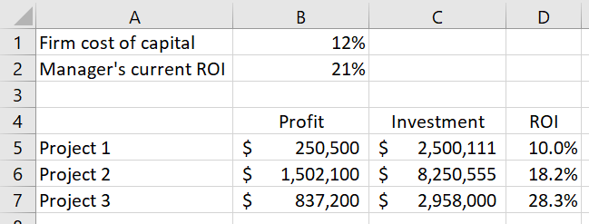
Using just return on investment, the manager would probably reject Project 1 and Project 2 and accept Project 3. The firm would prefer the manager accept both Project 2 and Project 3, since both projects have returns on investment well over the cost of capital.

10.4.3 Residual Income

To reduce the risk that managers turn down firm-preferred projects below their current return on investment, firms sometimes use residual income alongside return on investment. Both numbers might be tied to incentives, for example. (It is relatively rare to use residual income on its own to evaluate managers’ use of investment rights.)

A positive residual income means the profit from the investment is greater than the profits required by the cost of capital and the manager should invest in the project. A manager’s residual income increases with any project that has a return on investment greater than the cost of capital. This measure gives managers no reason to reject projects between their current return on investment and the cost of capital.

Firms could use a higher rate than the cost of capital if they are using this metric for stretch goals.

Let’s look at the earlier return on investment example with residual income added to the mix. (Again assume present values.)

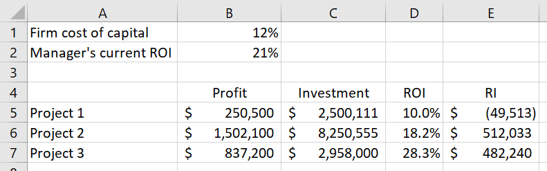
Now, assuming bonuses are at least partially based on residual income, the manager is more likely to accept both Project 2 and Project 3, since both projects would increase residual income and thus be personally profitable to the manager.

The problem with residual income is that it doesn’t scale in the same way return on investment does. It’s relatively easy to compare projects in a large department to projects in a small department using return on investment, since return on investment is expressed as a percentage. Comparing residual income from different size departments is more difficult to interpret.