8: Lean Accounting

Chapter 8 Guided Practice Problems

8.1 Lean Theory in the Cost Accounting Context

Cost accounting can be a victim of its own success. Through an array of cost accounting techniques that rationally evaluate the profit effects of discrete alternatives (Chapter 2), cost structure and continuous alternatives (Chapter 3), product costs (Chapter 4 through Chapter 6), and variances between actual and standard costs (Chapter 7), a cost accountant can tell managers a lot about how to maximize profit.

But these tools can backfire. A central assumption of cost accounting is that cost information should be the principal focus of managements’ time. Some factors that drive cost, however, also drive revenue. These factors include direct input quality, level of customer service, and product timeliness. Myopic focus on what drives the cost function can lead to the following.

• Managers targeting cost function drivers that also drive the revenue function.
• Managers not doing enough to target cost function drivers that do little to drive revenue.

Consider this modified version of the profit function.

The variables x₁, x₂, and x₃ represent factors that drive both costs and revenue. The overlap isn’t perfect, of course. The variables x₄ and x₅ only seem to drive revenue while variables x₆ and x₇ only seem to drive costs. If a manager in this firm focused solely on reducing costs (by addressing the drivers of cost), that manager would probably reduce the things that drove revenue as well.

Let’s illustrate this with an example.

Say x₁ represents the quality of direct inputs (e.g. direct materials quality and direct labor quality). Higher quality direct costs certainly does increase costs. It costs more to obtain high quality materials and high quality labor. A manager who only looks at these numbers will say, “Reduce the quality! Buy these inputs cheaper!” But, depending on where the firm is in the marketplace, input quality can also have a significant effect on revenue.

Who wants to buy junk that falls apart a few moments after the purchase?

The essence of lean philosophy (and thus lean accounting), is that the firm should distinguish between cost function drivers that simultaneously drive the revenue function and cost function drivers that do not. The latter is waste, and the firm should vigorously cut waste costs. At the same time the firm should be reluctant to cut non-waste costs.

The lean philosophy gets its name from the fact that it spends a lot of time cutting waste. Waste is anything that drives costs without driving revenue. Put another way, it’s activities the firm engages in that don’t bring any customer value.

I cover three general types of lean accounting techniques that help lean firms cut waste.

• Value stream income statements
• Costing for reduced inventory
• Costing for time-related waste

To be clear the lean firm also tries to control non-waste costs. It just has to be smart about controlling those costs, since there’s a significant risk that cutting those costs might also cut revenues. Most lean philosophers also advocate kaizen (or similar systems for continuous process improvement) to control non-waste costs in a conscientious way.

8.2 Value Stream Income Statements

8.2.1 The Value Stream

The value stream is what the company does to provide value to the customer. It’s typically a sequence—or stream—of activities that matter to the customer. It’s usually defined as the sequence of activities that starts with the customer placing an order and ends with product delivery.

Value stream: The sequence of activities required to bring the customer from order to delivery.

Here’s how the value stream ties into lean theory as expressed in Section 8.1. The firm exists to provide customer value, and the product features that drive customer value also generally drive the revenue function. So the value stream—which is where firm interacts with the customer—represents the part of the firm that’s most likely to affect customer value and most likely to have non-waste costs.

8.2.2 The Value Stream Income Statement

8.2.2.1 Disagreements in Practice

Lean firms often develop unique income statements that help them distinguish between costs that are directly related to the value stream and those that are not. Value stream costs are more likely to be non-waste costs. Non-value stream costs are more likely to be waste costs.

Sometimes these income statements are called plain language income statements or plain English income statements because they can be easier for non-accountants to understand.

There’s actually a surprising amount of confusion out there about what is and isn’t a value stream income statement. I believe this is because value stream income statements have several features, and some suggest that any income statement with even one of these features is a value stream income statement.

I disagree. For the purposes of this textbook, I mean something very specific when I talk about a value stream income statement. A value stream income statement is only a value stream income statement if it does all three of the following.

1. Does not use variance adjustments and only reports actual costs.
2. Separates value stream costs and non-value stream costs.
3. Adjusts for changes in raw materials and finished goods inventory.

8.2.2.2 Characteristic #1: No Variance Adjustments

In a full standard costing environment, the income statement first states costs at standard, then it states the variance adjustments. This setup can be difficult for non-accountants to understand.

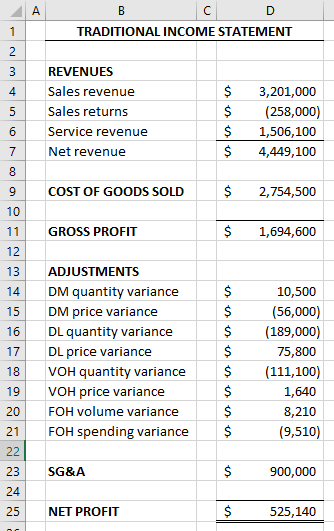
Value stream income statements record all costs at actual. This means no variances are collected or reported (managers compare actuals to budgeted amounts outside of the general ledger). Also, the firm often does not apply overhead. Instead it uses actual overhead costs incurred this period (insofar as those costs are relevant to the value stream).

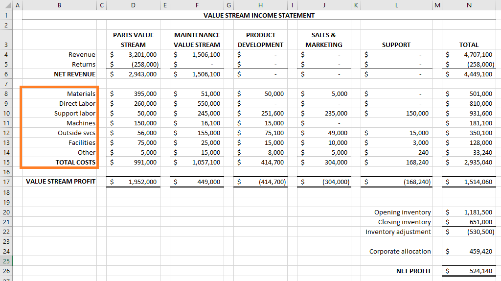
8.2.2.3 Characteristic #2: Separate Value Stream Costs

If a cost directly relates to the value stream, it is a value stream cost. It is relatively rare for lean practitioners to talk about the minutia of separating value stream and non-value stream costs. The distinction is supposed to be common sense and intuitive rather than technical and precise.

Here are some common examples of value stream costs.

• Material costs for material used in production for a product line
• Labor cost for workers assigned to the value stream
• Labor cost for support personnel assigned to the value stream
• Machine repair and maintenance for machines assigned to the value stream
• Outside services used by the value stream
• Proportion of facilities costs (e.g. factory lease, divided up by square footage of each value stream in the factory)
• Delivery costs for products in the value stream

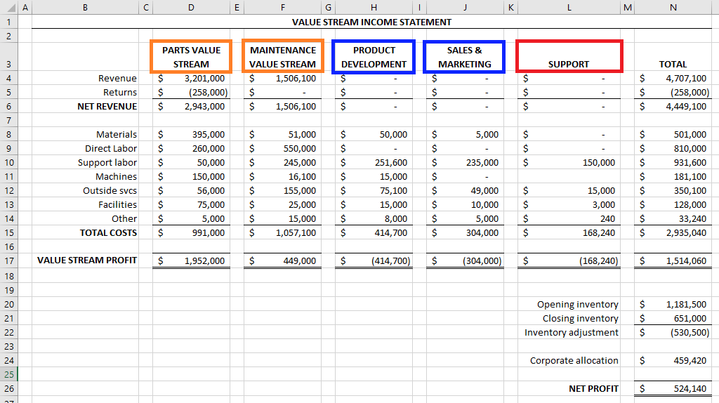
If the firm has multiple product lines, they can bundle these product lines into families and report each family’s value stream separately.

Sometimes a lean firm will also create additional quasi-value streams for non-value stream costs that sustain the business or product lines over the long term. Quasi-value stream is my name for it anyway. For example, a firm might have a quasi-value stream for new product development or a quasi-value stream for sales and marketing. These costs are not part of an order-to-delivery value stream but can be important revenue drivers in the long term.

The remaining non-value stream costs are reported as “support” costs or “other” costs. These costs deserve significant scrutiny because they do not directly relate to any value stream and have a relatively high likelihood of being waste.

Notice that costs are only traced to the value stream, not to individual product units. Lean firms often cut out systems that trace direct labor or direct materials costs to product units. They consider these systems to be waste.

Lean Similarities to Process Costing: Since lean firms trace costs to the value stream and not to individual product units, lean firms’ costing mimics process costing. Remember, from Chapter 6, that process costing is based on a very simple idea of dividing up costs evenly among all units. That idea gets more and more complex because of various complications, and the end result is process costing.

In a lean firm, though, process costing’s complications either (1) don’t apply or (2) are intentionally ignored for simplicity’s sake. You end up with a costing system that is relatively simple, like the initial costing system described at the beginning of Chapter 6. I discuss this more in Section 8.3.

8.2.2.4 Characteristic #3: Inventory Adjustment

Value stream income statements report on actual costs in the current period. But some of the cost of goods sold was incurred last period, assuming the firm has some inventory. So value stream income statements make an adjustment for change in inventory value. This adjustment is placed as far down the income statement as possible. That way income statement users have line of sight on what current period numbers are prior to the adjustment.

This adjustment increases expenses if inventory levels decrease and decreases expenses if inventory levels increase. This way the adjustment maps changes in inventory value on the balance sheet to expenses this period.

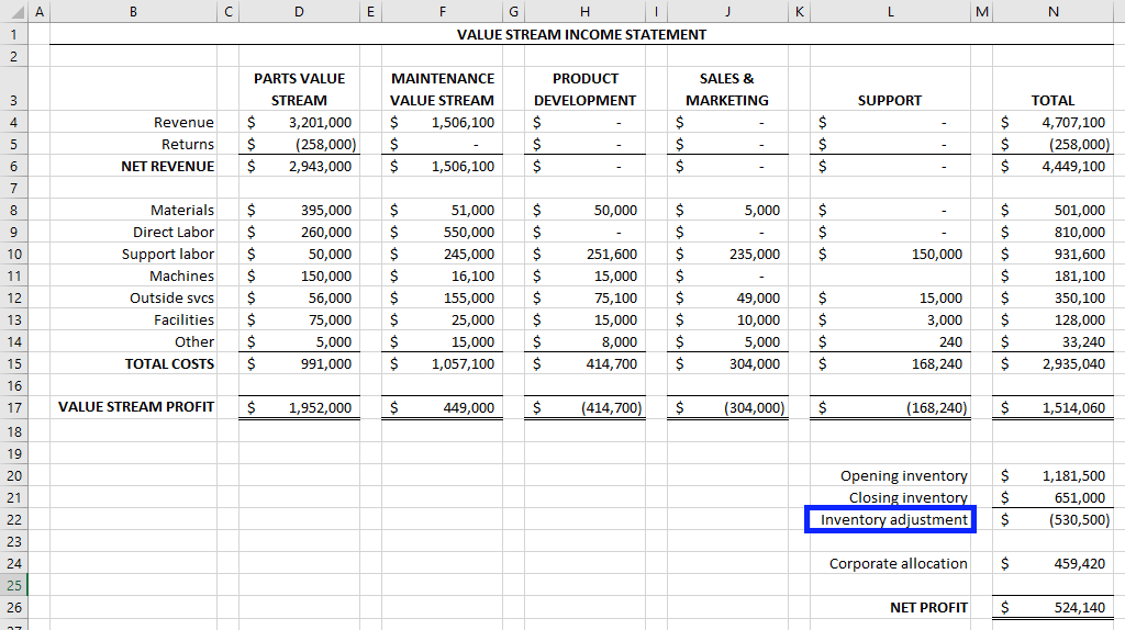
As I discuss in the next subsection, lean firms usually try to reduce their inventory until it is only enough to meet current customer needs. For many lean firms the ideal is to have no finished goods inventory on hand and to only order raw materials after an order is placed.

Perhaps counter-intuitively, this means that a recent-adopting lean firm likes to see a big expense on the inventory adjustment line. That means it is reducing inventory. Lean firms argue that this is a temporary effect and that long-term profitability significantly improves once inventory levels have been brought down.

Because the inventory adjustment line comes at the very end, the firm can still easily see its value stream profitability before that adjustment (cell N17 in the statement above). Lean firms often focus more on that number than on bottom line profit.

8.3 Reduced Inventory Accounting

8.3.1 Just-in-Time

Inventory is waste. That’s what lean says anyway.

The argument goes like this. Think about the last thing you bought. Did you ask the customer service representative how many items of raw materials or how much finished goods inventory the business had on hand before deciding whether or not to buy that good? Probably not. Storing large amounts of inventory (beyond what the customer needs right now) usually does not drive revenue.

But it does drive costs. Warehouse lease, warehouse utilities, warehouse security, transportation, obsolescence. These are all costs associated with raw materials and finished goods inventory.

Most lean firms adopt or move toward a just-in-time model of production. The firm reorganizes its production departments into atomized cells and work does not start on a product until a customer order is received. Once an order is received, a cross-trained team of workers in a fast, defect-free cell completes the product to exactly meets the customer’s needs (without over-delivering).

Just-in-Time (JIT): A philosophy of organizing firm processes that emphasizes fast, defect-free, cell-based production that only begins after an order is received.

When a firm adopts a just-in-time philosophy, it often uses backflush costing as a simpler approach to tracking costs.

8.3.2 Backflush Costing

8.3.2.1 Backflush as a Cost Accumulation Method

As discussed in Chapter 7 (using this handy illustration), there are a variety of questions to be answered by a cost accounting system. Backflush costing is one answer the question of cost accumulation method, i.e. where costs are accumulated. It is not an answer to the inventory valuation method question, i.e. which costs are considered product costs.

The backflush, per se, is a journal entry that credits cost of goods sold and debits inventory accounts. In a backflush costing system, actual costs are charged directly to the cost of goods sold account, and at the end of the period, the firm counts what few inventory items are left in process and “backflushes” costs to them.

Backflush costing, technically, can be paired with any inventory valuation rationale (two of which we focus on in this chapter: direct costing and throughput accounting). Backflush costing simply accumulates product costs, however the cost accounting system defines that term, in the cost of goods sold account until the end of the period, then backflushes those product costs to inventory accounts.

It makes sense for a just-in-time firm, where products are supposed to pass through manufacturing cells quickly and where are relatively few units left in inventory at the end of the period. A perpetual inventory system or even a periodic system that first debits costs to inventory accounts would be waste. The firm is just not interested in that information.

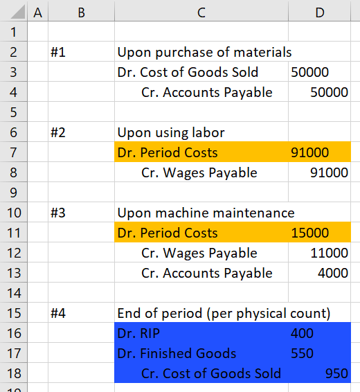
These are somewhat typical journal entries for backflush costing.

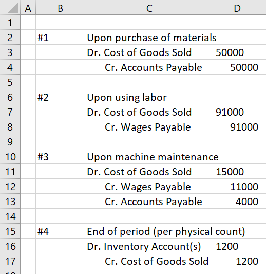
I was intentionally vague about which account is debited in entry #4 (see above figure). You might expect a debit to the raw materials inventory account or the WIP inventory account here. But many backflush systems combine these accounts into a “RIP” account. RIP stands for “Raw and In Process.” This account includes materials costs for raw materials still in the warehouse as well as direct materials costs for units in process. If the firm considers conversion costs to be product costs (which it might not, see the sub-section 8.4.2 below), then a separate “Conversion Costs” account is often used.

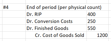
Rightly told, the final entry might look something like this.

8.3.2.2 Backflush vs. Process Costing

Lean firms’ penchant for simplicity leads a lot of them to use a simplified process costing system. In lean accounting, value stream income statements accumulate costs at the value stream level, much like process costing costs are accumulated at the department level (which is, effectively, the “process-level”). It’s a natural fit.

Hence, as with process costing, physical counts are often counted at the end of the period to determine how much to backflush to inventory accounts.

I said lean costing (i.e. backflush costing) is like a simplified process costing system. Here are some of the simplifying assumptions that might be used.

• Use physical counts of units instead of equivalent units, i.e. all units in process or finished are assumed to be 100% complete.
• This makes units the same for direct materials and conversion costs.
• Typically, weighted average is used instead of FIFO mindset. No need to give special consideration of BWIP costs since inventory carried over from period to period should be relatively small.
• Because the costs are aggregated at the value stream level, and a value stream takes the customer from order to delivery, there usually aren’t transferred-in costs (which process costing required to account for departments transferring units to one another before completing them).

Here’s a quick example.

If a firm considers direct materials, direct labor, and variable overhead to be product costs (more on this concept later), then it will simply take the average of these and determine a per unit cost. Let’s say total direct materials cost is $500,000, total direct labor cost is $450,000, and total variable overhead cost is $50,000. The firm counts 10,000 units (that includes both in process and completed units). Direct materials cost per unit is simply $50 (i.e. $500,000 / 10,000), conversion costs per unit is simply $50 (i.e. [$450,000 + $50,000] / 10,000) and overall cost per unit is $100 (i.e. $50 + $50).

Now, let’s say the firm counts $1,000 worth of raw materials in the warehouse at the end of the period and counts 120 units in process and 130 unsold units. It would create a backflush entry that looks like this.

Finished goods is debited $13,000 because 130 physical units times $100 of product costs per unit is $13,000. Raw and in Process are debited $7,000 because 120 units in process times $50 of direct materials costs equals $6,000, and that $6,000 plus the $1,000 of raw materials counted in the warehouse is $7,000 total. The debit to Conversion Costs is $6,000 because 120 units in process times $50 in conversion costs equals $6,000.

A firm might simplify this even further by not even backflushing actual costs. The firm might instead establish standards for direct materials cost per unit and conversion cost per unit based on its budgeted expectations before the period even began. Then it just uses those numbers to calculate the backflush entry. (Such a firm would review the standards from time to time.) This firm does not even need to calculate a new set of direct materials and conversion cost rates every period.

There are many variations possible, but they almost always favor the simple and non-technical over the complex and technical.

8.3.3 Direct (Variable) Costing

Earlier in the chapter, I wrote that lean firms often do not absorb overhead. This is because absorbing fixed overhead, provides a built-in incentive to overproduce. By “overproducing” I mean producing more WIP and finished goods units than there is demand for. Since lean philosophy views inventory as waste, many lean firms simply remove this incentive by not absorbing fixed overhead.

This is sometimes called direct costing or variable costing (these terms are interchangeable).

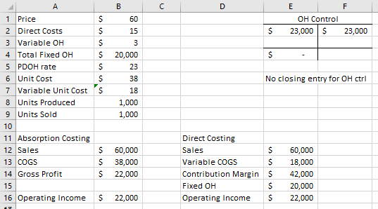
Consider the simple example below, where for simplicity I assume there are no SG&A costs and no ending WIP inventory. Budgeted production is 1,000, as is actual demand. This firm produces as many units as it sells (i.e. finished goods inventory levels remain constant). Whether the firm includes fixed costs in cost of goods sold via absorption or not, it produces the same operating income number (compare cells B16 and E16). This is only the case because the firm is not overproducing.

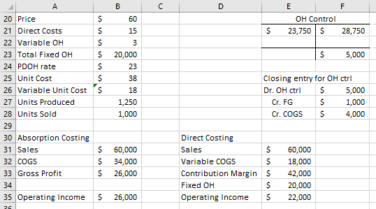
Now let’s assume the manager overproduces by 250 units (see cell B27 below). Perhaps the operating income above is just a few percentage points away from this manager’s bonus threshold. Overproduction is a way for the manager to make up the difference.

That’s because producing more units than demanded allows the manager to relocate some of the firm’s fixed overhead onto the balance sheet, where it is an asset. The fixed overhead costs applied to those 250 units sit in the finished goods inventory account instead of being expensed on this period’s income statement. Operating income in this scenario is higher under absorption costing but unchanged under direct costing (compare cell B35 and E35).

Now, let’s say the manager decides to overproduce by a lot: 1,000 units (see cell B46 below). The income number just keeps getting higher for absorption costing (see cell B54). Direct costing’s operating income is still unchanged (see cell E54).

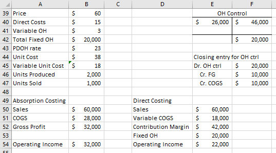
This is why many lean firms do not absorb fixed overhead. That is, they use  direct costing (at least on their internal reports, since GAAP requires absorption costing). This mitigates the incentive to overproduce that’s built into absorption costing.

Some firms go even further, as discussed in the next section.

8.4 Time-Related Waste

8.4.1 Capacity Waste

Capacity is a machine’s or person’s ability to do work (i.e. produce product units) within a given period of time. The degree to which capacity goes unused is Idle capacity.

Idle capacity is waste. It’s time-related waste, specifically. It drives costs but does not drive the firm’s revenue. It is an opportunity cost that is not reflected in traditional financial statements and cost reports. Lean practitioners see this as one of the shortcomings of traditional cost accounting.

But simply measuring total idle capacity does little to help a firm reduce idle capacity waste because there are many possible sources of idle capacity.

So, lean firms like to measure and report several different capacity numbers and look at the differences between these capacity numbers as a form of variance analysis. Overall idle capacity is sliced into actionable chunks that each have a unifying cause. Then the firm can go after each of these chunks of idle capacity, and their associated causes. That’s how they cut idle capacity waste.

To get these actionable chunks of idle capacity, firms define “capacity” in different ways, as shown below. By considering the differences between each of these definitions in capacity (from theoretical capacity all the way down to actual capacity) lean firms try to quantify the opportunity cost of idle capacity for each major cause of idle capacity.

• Theoretical capacity is a maximum theoretically possible work that a machine, team, and process can perform. It is based on the most ideal, even impossibly ideal, circumstances. There are 24 hours in a day, for example. Therefore, if each class meets for one-and-a-half hours a day, a student’s theoretical capacity for classes is 16 courses a semester. Sounds fun.
  • Theoretical capacity is almost always unreachable. Accidents happen, and unexpected circumstances arise. Machinery and people need time to rest, reset, recharge, and repair. In fact if the firm doesn’t allow for essential maintenance and downtime, those machine and people won’t last very long. But knowing the theoretical capacity is still useful: it allows the firm to contrast theoretical capacity and practical capacity.
• Practical capacity is the work a machine or person can complete in a given period of time assuming reasonably necessary rest and maintenance. The numerical difference between theoretical capacity and practical capacity can tell the firm a lot about how efficient their technology or workforce is. Less efficient technology or workers often lead to a bigger drop between theoretical capacity and practical capacity.
  • Even if companies can’t reach theoretical capacity, they still invest significant effort in minimizing the difference between practical capacity and theoretical capacity.
• Normal capacity is how much actual work is usually done by a machine or worker, as measured over the long term. Normal capacity might be the average actual capacity over the last few years, as long as that’s a long enough time frame to smooth out peaks and valleys from the firm’s natural business cycles.
  • When you interpret the difference between practical capacity and normal capacity, keep in mind the timeframe of normal capacity. It develops over a relatively long period of time. Assuming practical capacity has remained relatively constant across that same time, a significant difference between these two capacity numbers can reflect a strategic organizational problem. Something systemic in the firm is keeping it from realizing its potential productivity.
• Budgeted capacity reflects the expected work done for this period. Differences between budgeted capacity and normal capacity reflects recent changes in management’s mindset.
  • If budgeted capacity is greater than normal capacity, that might reflect management’s attempt to correct longstanding inefficiencies (such as those captured in the difference between normal and practical capacity).
• Actual capacity is the work that was done this period.
  • Differences between budgeted capacity and actual capacity reflect execution this period, as well as the quality of the budgeting process. (Actual capacity, of course, rolls up into normal capacity over time.)

From these five definitions of capacity, a lean firm can find four capacity variances (or “capacity waste” if you prefer). These names for these four variances come from Management Accounting: An Integrative Approach by McNair-Connolly and Merchant.

• Rate-based waste: theoretical capacity less practical capacity.
  • Over the long-term, the firm wants to reduce this variance by improving production technology so what’s practical gets closer and closer to the theoretical maximum for productivity.
  • For example, if the current machinery realistically needs 30% downtime (which means practical capacity is 30% lower than theoretical capacity), then management may consider an machinery upgrade that reduces this downtime requirement.
• Management policy waste: practical capacity less normal capacity.
  • Normal capacity is largely determined by policies and decision-making of a structural nature, and the degree to which it departs from practical capacity is a variance that should be pursued and minimized. This is often a strategy-focused variance.
  • For example, management decided over the long-term to target a market segment with limited demand. Thus the machinery has been in use over the last few years for less time than it could have been (i.e. less than practical capacity). A change in policy to target a larger segment of the market could reduce this waste.
• Budgeted waste: normal capacity less budgeted capacity.
  • This variance is very similar to management policy waste, but the time frame is smaller. Budgeted capacity is based on current best guesses and aspirations for a current or future period. Normal capacity is an average of the last few years. This could be a favorable variance if recent changes in manager mentality have sought to improve productivity.
  • For example, after considering its management policy waste, managers decide to budget higher capacity for the upcoming year, as part of their overall shift toward a bigger segment of the market. (This is a favorable variance, then!)
• Efficiency waste: budgeted capacity less actual capacity.
  • This variance captures the firm’s effectiveness at executing its plan. It is often driven by middle-level and lower-level personnel and operational decisions, rather than strategic or structural decisions.
  • For example, because of some problems adjusting the machinery to the new products (meant to appeal to a larger market segment), several large batches during the period were lost and actual capacity (i.e. actual production) was less than budgeted.

8.4.2 Throughput Accounting

8.4.2.1 The Theory of Constraints

Lean firms sometimes fight an uphill battle to compete with firms that maintain large inventories. Just think about whether you’d rather receive the product of your choice in a few hours (since it’s in stock) or in a few days (since the lean firm hasn’t started making it until you order it).

This puts a lot of pressure on a lean firm to be fast. This is one reason why the theory of constraints often goes hand in hand with lean enterprise.

The theory of constraints is a philosophy of how firms should maximize productivity, allowing for faster and less wasteful delivery. It focuses on the firm’s constraint (often called the CCR, meaning Capacity-Constrained Resources, or simply called the bottleneck). The constraint is the process that limits how many units the firm can produce within a given period of time.

This is similar to how water flow through a series of pipes is constrained by the narrowest pipe in the series. (Or, as a corollary, you do not need to collapse an entire hose if you want to stop water flowing through it. You can just kink one part of the hose and water flow slows or stops at that bottleneck.) Firms adopting a theory of constraints mindset identify, elevate, and optimize the constraint to make overall production as time-efficient as possible.

The theory of constraints, in doing this, helps eliminate time-based waste. Focusing effort on non-constraint processes can be an enormous and otherwise-invisible waste. Time is the ultimate constraint for all companies. All companies have only 24 hours in a day. Focusing on constraints, which limit how much can be done within the universal constraint of time, optimizes the firm’s production—according to proponents of that philosophy, at least.

The theory of constraints has implications for a firm’s accounting too. There are two important changes for our purposes: (1) it changes the firm’s backflushing entry, and (2) it changes constrained decision making (from back in Chapter 3).

8.4.2.2 Changes to Backflush Costing

As part of their analysis of the firm’s constraint, theory of constraint-practicing firms generally do not consider labor or overhead costs to be variable costs or product costs. Only raw materials are considered to truly vary with production (sometimes use the term totally variable costs to refer to costs that should be considered product costs, and it almost exclusively means raw materials).

Throughput Accounting: A system for accounting in which only raw materials are considered variable costs or product costs.

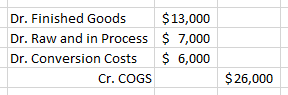
If the firm adheres to throughput accounting, the value of raw materials is the only cost that is backflushed into inventory accounts (RIP and finished goods). All labor and overhead are expensed in the period as operating expenses rather than through cost of goods sold.

In the spreadsheet below, I have highlighted how the backflush entries change because of throughput accounting.

8.4.2.3 Throughput Accounting Decision Making

Throughput, as an accounting term, is simply a modified form of contribution margin that follows the theory of constraints’ conception of what a variable cost is.

We can replace unit contribution margin with unit throughput in constrained resource decisions too. In fact, this is more accurate for constrained resource decisions. The emphasis on constrained resources comes the theory of constraints and make the most sense in the context of the assumptions that lead to throughput accounting.

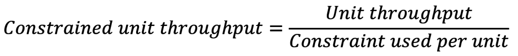
Now, just like in Chapter 3, the firm orders its products by constrained unit throughput, filling demand for each product from highest constrained throughput to lowest constrained throughput until there are no more units of the constraint left. Usually, the constraint is measured in units of time (i.e. constraint time used).

For additional coverage of how throughput accounting affects decision making, I suggest you read Thomas Corbett’s Throughput Accounting.