
Chapter 5 Guided Practice Problems
5.1 Activity-Based Costing Background
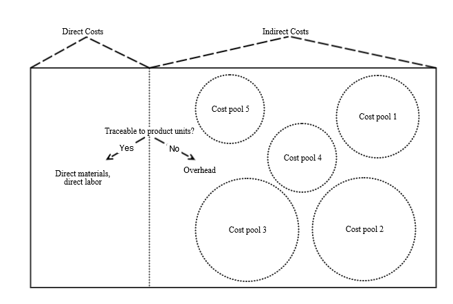
5.1.1 When is Job-Order Costing Inaccurate?
The correct answer is always. Remember that absorbing overhead costs to jobs is a fiction. It’s only an approximation of what overhead costs a job is actually responsible for.
I have a better question. When is job-order costing most inaccurate?
At the end of chapter 4, I said that a company-wide PDOH rate can be inaccurate when different departments have different styles of overhead. One department might have a lot of machinery-related overhead. Another department might have a lot of labor-related overhead. To solve this we developed departmental PDOH rates. Kumbaya, problem solved.
Except that it’s not solved. Although department PDOH rates can account for how product units cause different overhead costs from department-to-department, it ignores variation in how product units cause different overhead costs within a department.
- Different styles of product within a department. Even within a department different products might interact with overhead costs in different ways. One product might interact primarily with the department’s machinery. Another product might interact primarily with the department’s labor. If the firm has organizational reasons not to sub-divide departments any further than it already has, then using department PDOH rates won’t solve this problem. Overhead costs will be inaccurately applied to the two products.
Below I’ve created an example of this. It is a Powerpoint presentation turned into a video, with about 15 seconds on each slide (no narration). Of course, you can pause the video if it’s going too fast.
- Different relationships between volume and overhead within a department. Some overhead costs are closely related to volume while others are not. For example, some overhead costs are incurred each time a batch is started. If one product is produced in batches of 10 units and another product is produced in batches of 10,000 units, then the majority of batch-related costs really belong to the 10-units-per-batch product—it probably has many, many more batch-starts. Volume, meaning overall product units produced, for these two products might be exactly the same. Traditional job-order costing ignores the non-volume-related batch costs by relying on volume-related drivers like direct labor hours or machine hours.
I’ve created a video for this one too. It’s shorter overall and relies on details from the first video. It also has about 15 seconds per slide (still no narration).
So, the answer is that job-order costing is most inaccurate when the firm has multiple products that are (1) different enough to interact with department overhead in significantly different ways or (2) have significant costs that are not volume-related (like batch-related costs).
5.1.2 Activity-Based Costing Differences, Solving Job-Order Costing Inaccuracies
The whole point of activity-based costing (ABC) is to refine overhead absorption to make job-order costing more accurate. This is especially useful for firms with products that interact in substantially
Activity-based costing is very similar to job-order costing in a lot of ways. There are many permutations of ABC out there, of course. But the basic mainstream implementation of ABC follows much the same pattern you learned in Chapter 4: (1) product units are assigned any costs that can be directly traced to them, then (2) absorb overhead based on actual cost driver consumption and a pre-determined overhead rate.
But, of course, they are not the same thing. There’s a whole chapter’s worth of differences. ABC re-imagines some key aspects of the second step: overhead absorption. Here are three big differences between job-order costing and activity-based costing, based on ABC’s re-imagining of how to absorb overhead.
First, ABC uses unique terminology, which can lead to easily avoidable mistakes. Oftentimes, the new terms aren’t substantially different from terms covered in Chapter 4.
Second, firms using ABC subdivide overhead costs into sub-groups. Each sub-group of overhead costs is designed to capture a unique relationship between overhead costs and individual product units. Each sub-group of overhead costs uses a different cost driver to approximate its relationship. This is the main feature of ABC that makes it more accurate than job-order costing. These sub-groups can span multiple departments and/or capture sub-sections of overhead costs within a department. They are not limited by the company’s org chart.
Third, activity-based costing redefines all indirect costs (both overhead and SG&A) as “overhead” that can be applied to product units. This captures some SG&A costs that are actually related to individual product units, even if it is difficult to trace these costs to product lines. That said, ABC still uses an “other” sub-group of costs, which are not absorbed by product units and are instead expensed in the period they’re incurred. ABC just uses different criteria (different from traditional job-order costing) to decide which costs are product costs and which are period costs.
5.2 Activity-Based Costing: How Does It Work?
5.2.1 Terminology
Overhead: any cost that is not directly traceable to individual product units (includes SG&A).
Activity cost pool: a sub-group of overhead costs that share a common relationship to product units. Sometimes this is just called a cost pool.
Activity driver: a cost driver that approximates the relationship between an activity cost pool and product units.
Activity rate: a PDOH rate for a particular activity driver and activity cost pool.
$$\Large Activity\ Rate= \frac{Budgeted\ Activity\ Cost\ Pool}{Budgeted\ Activity\ Driver}$$You can see why “activity” is in ABC’s name, since the word is used in just about every term!
The theory for ABC basically goes like this. A firm performs various activities to add value to the finished product, and each activity has a unique set of overhead costs associated with it. These overhead costs are that activity’s cost pool. A unique activity driver is theorized to approximate the relationship between each cost pool and each product unit.
5.2.2 Implementing ABC
The mechanical process of ABC takes place in two separate allocations. That means the firm moves costs twice.
First, the firm separates overhead costs into cost pools, moving them from where they actually originate into the cost pools. This is the first-stage allocation. Second, the firm applies costs from cost pools to individual product units based on each individual product unit’s consumption of the activity driver. This is the second-stage allocation.
At first blush this looks easy. The second step is basically the same procedure as job-order costing with department PDOH rates: applying overhead to individual product units through multiple PDOH rates. The first step might also seem easy on the surface as well.
But it isn’t easy. Dun, dun, DUUUUUUN!!
See, determining which costs go to which cost pool—or even deciding which cost pools to create—is something that requires a lot of professional judgment and/or well-refined data.
Say a firm wants to implement ABC. It often contracts with a consulting firm that specializes in ABC. Some well-paid ABC consultants fly in, interview workers and managers, statistically measure overhead costs’ inter-relationships using various activity drivers, and attempt to balance the need for more cost pools (for increased accuracy) and the need for fewer cost pools (for parsimony).
Their time and expertise usually isn’t cheap, and most of that effort is time-intensive and expertise-intensive. Only then do you have cost pools to break costs up into. Then, you can start to do the first-stage allocation.
How?
5.3 Activity-Based Costing Example
Let’s assume the firm has three sources of overhead costs. These are all budgeted numbers.
- Shop supplies: $50,000
- Machine maintenance workers’ wages: $120,000
- Miscellaneous administrative costs (e.g. CEO salary, office supplies): $85,000
ABC consultants decide the firm performs effectively two activities that add value: machining and finishing. They create the following table to express the relationship between overhead sources and these two activities. Of course, there’s also an “other” category, where the firm can place overhead costs that really do not relate to product units. So, I guess there are three activity cost pools in this example.
| Shop Supplies | Maintenance Wages | Miscellaneous Administrative | |
| Machining Activity | 50% | 90% | 5% |
| Finishing Activity | 35% | 10% | 20% |
| Other (Activity) | 15% | 0% | 75% |
| TOTAL | 100% | 100% | 100% |
From this table, you multiply each percentage by the total budgeted cost to get the following table. The far-right column gives the cost that should be allocated to the three cost pools.
| Shop Supplies | Maintenance Wages | Miscellaneous Administrative | TOTAL | |
| Machining Activity | $25,000 | $108,000 | $4,250 | $137,250 |
| Finishing Activity | $17,500 | $12,000 | $17,000 | $46,500 |
| Other (Activity) | $7,500 | – | $63,750 | $71,250 |
| TOTAL | $50,000 | $120,000 | $85,000 |
It is costly to (1) come up with the cost pools, (2) determine how much overhead cost goes into each cost pool, and (3) update the cost pools and first-stage allocation numbers over time. Thus ABC usually isn’t implemented by smaller firms or firms that don’t have especially inaccurate job-order costing numbers (see Section 5.1).
Once the firm has these budgeted cost pool numbers (the right-hand column in the table above), it divides those numbers by the respective budgeted activity drivers. For this example, let’s assume the two cost pools are based on the cost drivers of machine hours for the machining activity and batch-starts for the finishing activity.
The firm estimates it will have 5,000 machine hours next period and 500 batch-starts.
$137,250 budgeted machining cost pool / 5,000 budgeted machine hours = $27.45 per machine hour.
$46,500 budgeted finishing cost pool / 500 budgeted batch-starts = $93 per batch-start.
These are our two activity rates. The “other” category does not have an activity driver or activity rate and is considered a period cost.
As product units consume these drivers (machine hours or batch-starts), overhead cost is allocated to those product units using these two activity rates. (The batch-level cost is most likely split evenly across all units in a batch.)
Let’s assume product unit OP57 consumes 6 machine
Product unit OP106, however, consumes 2 machine hours and is part of a batch of 3 product units. The firm would allocate $54.90 in machining costs and $31 in finishing costs, for a total overhead allocation of $85.90.
Typically, most product units receive at least some overhead cost from each cost pool. But if the firm’s products are different enough to justify using ABC, then the amounts allocated from each cost pool probably vary significantly from product line to product line and from product unit to
SIDE NOTE: Technically, ABC can be used with a process costing system (which we’ll talk more about in Chapter 6). A process-costing-based ABC system would just charge activity rates to processes or departments instead of charging those rates to jobs or individual product units.
That said, in this chapter I present ABC as an offshoot of job-order costing because ABC’s usefulness at the process-level is decidedly muted. Much of the usefulness of ABC comes from its ability to pick out the idiosyncratic consumption of resources of different jobs, and that is much less likely to happen in a process costing situation.
5.4 Activity-Based Management
5.4.1 What is Activity-Based Management
Activity-based costing more accurately measures unit cost. In Chapter 1, I said managers want to know who or what is responsible for costs the firm
Therefore, the result of ABC’s increased accuracy is that managers can make an array of decisions better. This includes the decisions covered in Chapters 2 and 3. It also includes some new ones. When managers take advantages of ABC’s more accurate picture of costs to make improves decision making is called activity-based management.
5.4.2 Non-Volume-Related Overhead Costs
To fully understand the scope of activity-based management, I need to expand on my earlier description of activity-based costing.
At the beginning of the chapter, I illustrated the difference between volume-related and non-volume-related costs by pointing out that batch-related costs are not strictly volume-related. There are other types of costs that are not volume-related. ABC usually splits up overhead costs at several levels. (Direct materials and direct labor are product unit-level costs by definition.)
- Product Unit-level: overhead costs that are driven by volume. For example, factory supplies, nuts
and bolts, machine lubricant, maintenance overtime, a portion of utilities, etc. - Batch-level: overhead costs that are driven by batches produced. For example, equipment testing, cleaning, and set-up, batch transportation across factory floor, purchase order placement, etc.
- Product Line-level: overhead costs driven by producing a particular product line. For example, research, development, and product testing, product launch (including advertising), some manager/supervisor salaries, some administrative staff salaries, etc. This can also include costs driven by customer maintenance and loyalty, such as overhead costs from sales calls, account maintenance, and loyalty programs. This level can also include design costs and engineering salaries. Some companies break out these costs as a separate level.
- Organization-sustaining-level: overhead costs driven by being in business, in general. For example, some administrative costs, information technology costs, accounting
and reporting,
All levels listed above, except the first, tend to be non-volume-related.
Think about it. If all you know about a firm is that it has high volume, does that mean the firm always has a lot of batch starts, product lines, and customers? What if all you knew was that the firm has low volume? Does that firm always have few batch starts, product lines, and customers?
The answer is no. A firm can easily have low volume and still have a lot of batch starts (i.e. small batches), product lines (i.e. a range of specialized product lines), and customers (i.e. a lot of small customer accounts). And vice versa.
You need to understand the full array of non-volume-related overhead costs if you’re going to understand the power of activity-based management in the below decisions.
5.4.3 Customer Profitability Analysis
Firms using ABC should better know the true profitability of each customer too, mainly because the firm has a better picture of the type of batch-level and product line-level overhead costs each customer is causing the firm to incur.
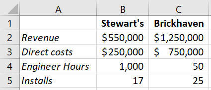
As an example, Build Boise, Inc. produces custom software in the western United States. The firm uses activity-based costing and wants to compare the profitability of two customers: Stewart’s, LLC and Brickhaven International. Build Boise, Inc. uses five activity cost pools based on four activities: research, design, quality, and other.
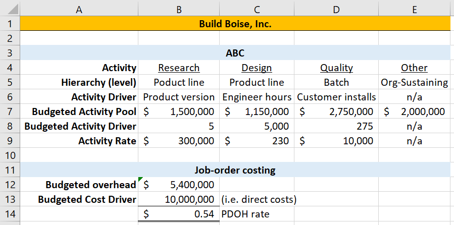
As shown below, the two customers of interest use Build Boise’s services in unique ways. Neither requires a new product version, but they do require varying levels of re-design (i.e. design activity) and quality control (i.e. quality activity). This is in addition to each customer’s direct costs, in the form of licensed portions of Build Boise’s software.
In the below table, I use job-order costing and activity-based costing to estimate these two customers’ profitability. Under job-order costing Stewart’s, LLC is more profitable than Brickhaven International, and both seem to be profitable. Under ABC the picture comes into better focus. Stewart’s, LLC is not only less profitable than Brickhaven International but unprofitable altogether.
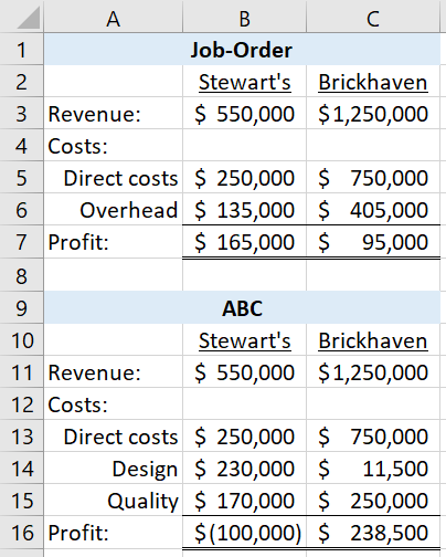
Build Boise, Inc. would most likely respond to this new information by negotiating for a more profitable contract from Stewart’s, LLC. If that does not work, the firm might be better off
Build Boise, Inc. can also trace this unprofitability to its cause: the intensive design work required by Stewart’s, LLC. They consume 1,000 engineer hours, a fifth of the annual budget for engineer hours. Build Boise, Inc. can use this information to identify other likely unprofitable customers or to screen unprofitable potential customers. It might re-evaluate how much it is willing to customize software for customers. Or it might try to re-design its processes or offerings to reduce the cost of engineer hours.
5.4.4 Product Mix and Process Improvement Analysis
Analysis very similar to the above might help Build Boise, Inc. improve (1) the products and product mix it offers or (2) the processes it uses to provide these products. Let’s look at an example of each of these. (I’ll use the same activity cost pools and rates for Build Boise, Inc., shown above).
5.4.4.1 Product Mix Analysis
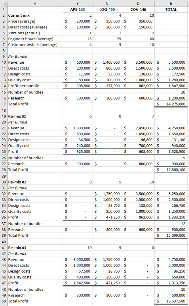
First, Build Boise, Inc. might change its product offerings or product sales mix. (Decisions to change product offerings or product sales mix overlap so much that I consider them together in this section). Consider the following scenario for Build Boise, Inc. Based on the sales department’s projections, the firm could re-mix three of its most popular products into three alternative configurations, i.e. re-mixes.
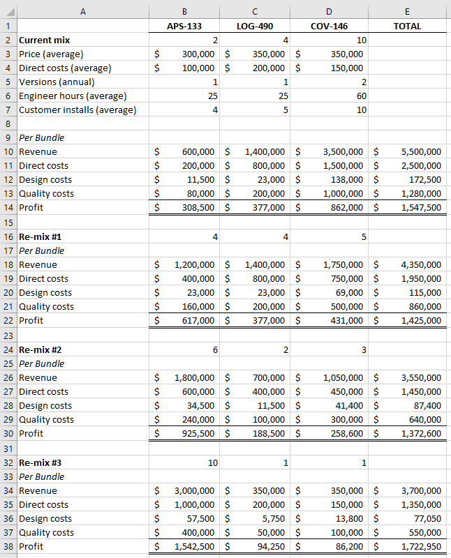
(I simply assume the same number of bundles are sold in each scenario, so I can evaluate the profit of these re-mixes on a per bundle basis.)
Because the firm has ABC information on these three products, it can easily evaluate the profitability of each of these re-mix scenarios. Notice that I omit overhead costs related to the research activity. That’s because this decision does not involve dropping any of these product lines, as a whole, meaning the cost of annual versions for each product will stay the same.
Now, let’s consider additional possible mixes that drop one or more of the products being offered. For this calculation I include research activity costs and the number of bundles sold, so I can evaluate the re-mix scenarios on a total profit basis (as opposed to the profit-per-bundle basis used above).
5.4.4.2 Process Improvement Analysis
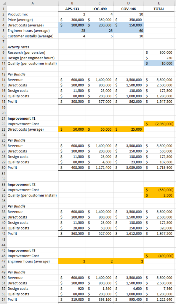
Second, ABC can help the firm evaluate potential improvements to its processes. Process improvements can cost a lot. ABC information can often give the firm more accurate information about the profitability of these improvements.
For example, look at three different improvements below (relevant original items highlighted in blue, with changes highlighted in orange). Improvement #1 reduces direct costs. Improvement #2 streamlines quality checks, reducing cost per customer install. Improvement #3 involves hiring better engineering staff, reducing how many engineer hours each product consumes.
5.4.5 Pricing Decisions
5.4.5.1 General Pricing Decisions
Pricing philosophy varies from firm to firm. Some firms look to the market to set the price (more on this in Chapter 8). A lot of other firms price their products based on how much they cost the firm. This is actually a more traditional view. Many prices have to be set in markets where the price is less than clear, or over a time-horizon that makes it economically risky to rely on current market prices.
ABC can improve prices set on product cost because it can improve the firm’s understanding of
5.4.5.2 Cost-Plus Contracts
Prices based on product cost often use full absorption cost (which thus includes applied overhead) plus a fixed profit margin (as a percentage) or a fixed unit profit (as a dollar amount). Long-term contracts are often made on this basis. These are called cost-plus contracts because the firm is reimbursed for costs, plus a little extra as profit.
Cost-plus contracts are used because long-term project costs can be difficult to estimate beforehand. They also have the advantage of mitigating some perverse incentives. Setting a fixed overall contract amount, as opposed to a cost-plus contract, can motivate the seller to cut costs in an unacceptable way, since this will maximize short-term profits.
For cost-plus contracts, overhead reimbursement is the trickiest part. Direct costs, by definition, are relatively easy to trace and reimburse. Fixed profit margins or dollar amounts are also relatively easy to calculate and are determined by negotiation at the beginning of the contract. Overhead costs, though, can be a source of disagreement because they are only applied to individual product units. How much overhead each product unit is actually responsible for cannot realistically be known.
Therefore much of the work in negotiating a cost-plus contract involves measuring and negotiating the selling firm’s overhead rate. Activity-based costing can improve these measurements and negotiations. The buying firm has more peace of mind that applied overhead amounts are not arbitrary. The selling firm has more peace of mind that it will be fairly reimbursed for overhead costs it really has incurred.
5.5 Simplifying ABC
5.5.1 Why Simplify ABC?
Implementing ABC can be costly. Some of that cost comes simply from its complexity. The firm has to study, analyze, record, and keep up to date a multitude of drivers as well as the relationships between overhead sources and those drivers.
Complexity as a cost is sometimes overlooked, and it’s useful for you to get in the habit of identifying it when considering the profitability of different alternatives. As the firm’s operations get more complex, you need to hire higher caliber people to deal with the complexity (or suffer the costs of higher turnover), you likely have to purchase more robust software, and you might have additional compliance costs (lots more billable hours are incurred determining complex legal positions than straightforward ones).
This section covers two different ways of simplifying ABC, one of which simplifies first-stage allocation and one of which simplifies second-stage allocation.
5.5.2 Time-Driven Activity-Based Costing (TDABC)
5.5.2.1 TDABC Procedure
Time-driven activity-based costing, as the name implies, uses time to simplify ABC. It’s especially useful for service firms, where time spent by professionals is what adds value and can be very important to how much overhead cost is incurred.
Here’s the procedure (don’t worry, I’ll have an example and additional explanation later in this section).
- Calculate a capacity cost rate. This is the cost of time at the department or process. That is, it is total overhead cost for the department divided by total practical capacity in the department. (Practical capacity is explained further in Chapter 8.) Practical capacity, for TDABC purposes, is always measured in time, such as doctor hours, nurse hours, engineer hours, etc.
- Determine how much practical capacity (in hours) is consumed by each unit of activity driver. This is what the TDABC consultants come do, i.e., I’ll need to give you this number if asking a test question. This is the practical capacity (in hours) that it takes for the department to perform one unit of the activity driver. I’ll call this number practical capacity per activity driver.
- Calculate activity rates by multiplying the capacity cost rate by the practical capacity per activity driver. You then use these activity rates as you would in standard ABC for the purposes of second-stage allocation.
Here are a few things to notice about this procedure.
- This procedure eliminates the need for a first-stage allocation percentage table that correlates each activity cost pool to each source of overhead.
- Overhead cost is pooled at the department/process level. This means that how finely you define the department/processes used in TDABC will play a role in the accuracy of the TDABC system. This also means there’s at least some level of assumption that overhead cost is incurred the same way for all units that pass through a department/process.
- TDABC is similar to Chapter 3’s constrained decision making. Both calculations use denominators that measure the constraint: total practical capacity for TDABC and per unit consumption of constraint for Chapter 3.
5.5.2.1 TDABC Example
Here is an example.
Let’s assume there’s just one department and this department has the same three sources of overhead cost as the earlier example (see Section 5.3). These are the costs per period.
- Shop Supplies: $50,000
- Maintenance: $120,000
- Misc. Administrative: $85,000
Now assume the department has, given reasonable assumptions about time off, breaks, and downtime, a certain number of mechanic hours per period: 2,000 mechanic hours. This is the department’s practical capacity.
The capacity cost rate for this department is simply total overhead cost divided by practical capacity.
(50,000 + 120,000 + 85,000) / 2,000 = $127.50 overhead cost per mechanic hour
Now let’s assume, unlike in Section 5.3, that the firm has two activities it has identified: machining and finishing. I’ve removed the “Other” activity for simplicity (and a TDABC firm is likely to simply exclude such period costs from the numerator of their capacity cost rate calculation). Machining is still driven by machine hours and finishing is still driven by batch-starts.
The firm conducts some analysis and determines that each machine hour consumes 1.25 mechanic hours and each batch-start consumes 0.75 mechanic hours. These numbers are the “department time per activity driver units” that I referred to in my initial run-down of the TDABC procedure.
Now the firm will just multiply (1) capacity cost rate by (2) department time per activity driver unit. That gives you activity rates (I’ve rounded to cents below).
1.25 * $127.50 = $159.38 overhead cost per machine hour
0.75 * $127.50 = $95.63 overhead cost per batch-start
From there, the firm would complete second-stage allocation as it would in traditional ABC: multiplying each rate by the job’s or product unit’s consumption of each activity driver to get the overhead cost of that job or product unit.
5.5.3 Approximated Activity-Based Costing
5.5.3.1 Approximated ABC Procedure
Some firms that use ABC create many activity cost pools and many activity drivers. Hundreds. Managing this system can be quite cumbersome.
Importantly, this complex kind of ABC system can be simplified by only performing second-stage allocation using the biggest activity drivers.
Here is the procedure.
- Determine the activity cost pools with the highest dollar value. If you have twenty activity cost pools, you might pick the five activity cost pools with the highest dollar value. I’ll call these high-dollar cost pools, while all those cost pools you don’t select are low-dollar cost pools.
- Calculate the total cost of your high-dollar cost pools. Then, separately, calculate the cost of your low-dollar cost pools (these totals are important for the next step). Now you have total high-dollar costs and total low-dollar costs.
- Proportionally redistribute all dollars from low-dollar cost pools to high-dollar cost pools. Use the equation below. (The “HighDollar Pool” refers to a generic high-dollar cost pool. Repeat this calculation for each high-dollar cost pool).
Now you can calculate activity rates for the high-dollar cost pools (dividing each new “xyz cost pool” by its budgeted activity driver). Then complete second-stage allocation as normal, except you’re only applying costs to jobs with the high-dollar cost pool activity rates.
If you have appropriately chosen your low-dollar and high-dollar cost pools, this approximate method is easier to maintain (fewer activity drivers to measure and update) while still providing relevant information for decision makers. Often an approximated ABC system can provide cost figures that only slightly deviate from the cost figures of a full ABC system that uses all activity drivers available.
5.5.3.1 Approximated ABC Example
For simplicity, I will continue with the ABC example from earlier, even though it only has three activity cost pools. This is not what it looks like in practice, but it will keep the example simple. Here, in the far-right column, are the results from first-stage allocation (see Section 5.3).
| Shop Supplies | Maintenance Wages | Miscellaneous Administrative | TOTAL | |
| Machining Activity | $25,000 | $108,000 | $4,250 | $137,250 |
| Finishing Activity | $17,500 | $12,000 | $17,000 | $46,500 |
| Other (Activity) | $7,500 | – | $63,750 | $71,250 |
| TOTAL | $50,000 | $120,000 | $85,000 |
Let’s assume the company is not interested in maintaining the Finishing activity. Thus, Finishing is our only low-dollar activity cost pool. Usually there are more than one such low-dollar cost pool, and we need to sum them to arrive at total low-dollar cost. In this case, the Finishing cost pool costs (i.e. $46,500) are also our total low-dollar costs.
The firm will need to redistribute the total low-dollar costs of $46,500 to Machining and Other (since those are our high-dollar cost pools). Total high-dollar cost is $137,250 + $71,250 = $208,500. We can calculate the new Machining and Other cost pools as follows.
Machining: 137,250 + 46,500 * 137,250 / 208,500 = 137,250 + 30,609.71 = 167,859.71
Other: 71,250 + 46,500 * 71,250 / 208,500 = 71,250 + 15,890.29 = 87,140.71
Our new activity rate for the Machining activity (assuming the firm budgets 5,000 machine hours, same as in Section 5.3) is $167,859.71 / 5,000 = $33.57 per machine hour. We will allocate costs to jobs using this new rate, and get an approximation of what we would have calculated with the full system.
Given that we only have three cost pools in this rudimentary example, the approximate system might be significantly different. But if this were a situation with many cost pools and if we chose highly significant cost pools from among them, the differences might be relatively small.