
Also, will Marco Polo ever find Marco Polo? Tune in next week for the exciting conclusion.
(Public domain image)
Chapter 4 Guided Practice Problems
4.1 Firm Types
4.1.1 Three General Types of Firms
Last chapter, I discussed how managers refine their understanding of the firm’s cost function by dividing up costs based on the cost’s behavior: variable costs versus fixed costs. This chapter I discuss how managers refine their understanding of the firm’s cost function by dividing up costs based on the cost’s location. Actually, determining a cost’s location is the premise for Chapter 4 through Chapter 7.
But first I must comment on different firm types. You could say that there are three types of firms.
- Merchandising firms: these firms buy products from a manufacturer or wholesaler, then re-sell those goods (making few if any changes to the products) to consumers. Customer value from a merchandising firm is the convenience and availability of goods that the consumer otherwise has no access to. Merchandisers are, by definition, “the middleman.”
- Service firms: these firms typically do something that is useful to a client. That often means the service firm provides expertise that the client does not have, i.e. expertise is the basis for customer value. These firms often have few if any physical products that clients take home with them.
- Manufacturing firms: these firms take raw materials, perform some sort of process that changes these raw materials into something more useful to customers, then sells the finished goods to wholesalers, to merchandisers, or directly to customers. Manufacturing firms usually produce a physical product the customer is buying, which includes software (software is just a expertly-arranged set of electrons that are captured on some medium).
The principles of cost accounting discussed up until now are almost universally applicable to firms of all three different types. But Chapter 4 through part of Chapter 7 primarily targets manufacturing firms. A lot of this information is useful to service firms as well.
4.1.2 Cost Issues in Merchandising Firms
Merchandising firms don’t really use job-order costing, activity-based costing, or process costing, which are the basis for the next few chapters. A merchandising firm does not need to spend as much time sorting out the location of costs because their costs are relatively easy to locate: a product’s cost is its purchase price from the wholesaler. Maybe you can add freight to that. Maybe one or two other exceptions. Otherwise it’s pretty simple.
Most of merchandising firms’ effort to maximize profit uses a Chapter 3 mentality. Let me explain that here. Here’s a key expression of the profit equation from Chapter 3.
$$\Large \pi = pq-vq-f$$If a merchandising firm wants to maximize π, it can do one of four things: maximize p, maximize q (assuming p > v), minimize v, or minimize f. Merchandising firms’ cost accounting behavior lines up with those four mathematical ideas remarkably well.
First, some merchandising firms choose a differentiation strategy, which means they try to maximize p. Examples of this are Tiffany’s or Williams Sonoma. They want the products they sell to seem high quality simply because they’re sold at their stores, which lets them charge a higher price. Presumably a firm pursuing this strategy would increase prices more than their variable costs increase. So they need to keep a close eye on their variable costs as well (i.e. cost accounting information). Tiffany’s is very aware of how much its products cost and tries to ensure its high-cost items are those that will fetch a high price.
Second, merchandising firms like to maximize q. They look for what’s doing well on the market. They try to either stock those goods ahead of time (in anticipation of demand) or they build supply chains that are nimble enough to react (as demand surges or changes in an unexpected way). Did someone say “Chewbacca mask?” Stocking in anticipation of demand requires a lot of budgeting and cost accounting information so as to determine warehousing costs and transportation costs. Nimble supply chains require information about suppliers’ costs and capacity costs.
Third, merchandising firms try to minimize v. This is what Walmart does through its massive, global supply chain and its leverage over manufacturers. By decreasing the variable cost it pays, it can lower prices and get customers to come to Walmart instead of its competitors. That sounds like a Walmart commercial because Walmart often just explains their business model on their commercials.
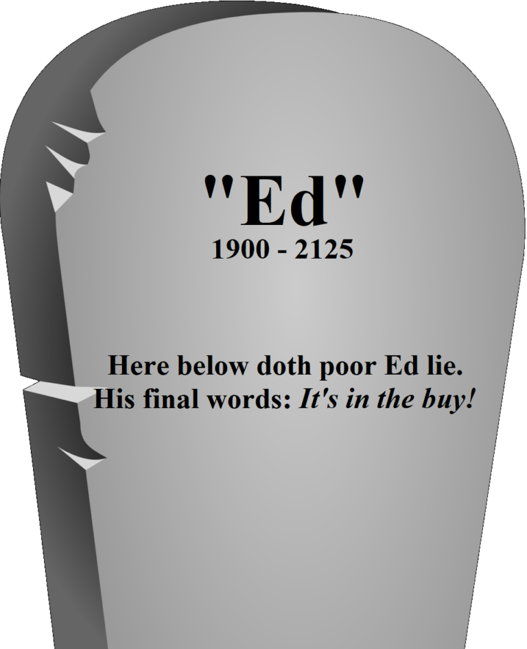
I once heard of an exemplary merchandiser, named Ed, who wanted something like this on his tombstone.
A merchandising firm succeeds or fails, in large part, based on what it is buying from suppliers and at what price. That’s v in our profit equation, and it sets the floor for how much the firm can resell that product for. Merchandisers spend a lot of effort finding information that gives them an advantage in driving down v, often through understanding the cost of space in the store and in understanding the cost functions of their suppliers.
Fourth, merchandising firms minimize f. At least, they do nowadays. Look at Amazon. One reason to their success is that they do not have brick-and-mortar stores like a traditional merchandising firm. Those brick-and-mortar stores are huge fixed costs. By minimizing f, Amazon can ensure that more and more of its sales go toward profit, which it then reinvests in additional and more convenient offerings. Also, it can ride the waves of demand better because it is not burdened down by massive fixed costs (i.e. the low DOL/low CM ratio strategy) that might otherwise sink a company during a sales dip.
Many merchandising companies are not just merchandisers. Walmart and Amazon are manufacturers and/or service providers as well. Walmart licenses or develops in-house a slew of Great Value brand products. Amazon develops some of its own shows for Amazon Prime. Walmart and Amazon both have credit cards and at least some financial services they offer (financial services are services).
So even if you’re certain that you’ll work for a merchandising firm, don’t go to sleep yet. A lot of these firms still need to make critical manufacturing and service decisions because there are parts of the company that act just like mini-manufacturing or mini-service firms.
4.2 Cost Characteristics: Cost Location, Responsibility, and Traceability
4.2.1 Location, Responsibility, and Traceability
As I talk about costs, let me channel a real estate agent: location, location, location!
In Chapter 1 I said that managers want to know who or what is responsible for costs so they can hold these people or things accountable for them (see second half of section 1.2). When I say cost location, I mean the location of the cost within the company, including who or what is responsible for it. Sometimes the ability to determine a cost’s location is called the cost’s traceability. Tracing costs means finding out where they’re located, which is tantamount to finding out who’s responsible for them.
Physical proximity, or location, is actually a very common way of determining who or what is responsible for a cost. If a cost comes from certain factory, then it was probably incurred because of the products made at that factory. If a cost comes from an engine block located inside a particular car that rolled off the assembly line, then the cost of that engine block cost was probably incurred because of that particular car being assembled.
Yes, sometimes physical location does not line up with causation. There are certainly exceptions. A lot of these exceptions are services provided by another department within the company. The IT department, for example, might incur a lot of labor cost due to overtime as it redesigns the computer system for a particular factory. The IT department might do most of that work while located far away from the factory, even though these costs are caused by the factory. Many companies account for this with interdepartment cost allocations, which I cover in Chapter 10.
4.2.2 Direct and Indirect Costs
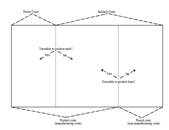
This is where most textbooks use the term “cost object.” Full-body shiver. What a mess. They’ll tell you a “direct cost” is a cost that can be traced to the cost object and that an “indirect cost” is a cost that cannot be traced to the cost object. By defining the term cost object so broadly, these textbook authors allow for the cost object to be all sorts of things: product units, product lines, departments, teams, customers, etc.
Theoretically that’s true. It’s also largely unnecessary. In a manufacturing firm there’s really only one cost object worth defining: products. The question of cost location, then, is “Can this cost be traced to individual product units?”
I’m just going to say costs are direct or indirect based on this one question because that gives us all the terminology required for this textbook. If I need to talk about costs that trace to teams, individuals, customers and so forth, I’ll use different wording.
Direct costs: costs that can be traced to individual product units.
Indirect costs: costs that cannot be traced to individual product units.
4.2.3 Product and Period Costs
There’s also a second question that’s important too. In a manufacturing firm, you want to know the cost of manufacturing certain product lines. In a merchandising firm, you want to know the cost of selling certain product lines. In a service firm, you want to know how much a certain service line costs. If you don’t know these things, you cannot make keep-or-drop decisions.
Said differently, you want to know product costs. For GAAP you need to know product costs because you inventory product costs, compared to period costs that you expense in the period they’re incurred. I’m going to use the term “product costs” more loosely than GAAP would like, but the general idea is the same.
Product costs: costs that can be traced to a particular product line.
Period costs: costs that cannot be traced to a particular product line.
In a manufacturing firm we often replace these two with terms that have the word “manufacturing” in them. Because we’re manufacturers, huzzah!
Manufacturing costs: product costs in a manufacturing firm.
Non-manufacturing costs: period costs in a manufacturing firm.
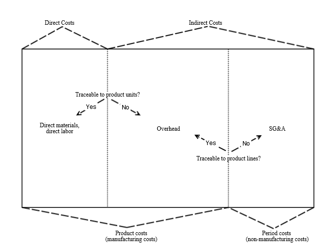
I show this in the below figure. Generally, more traceable costs are to the left and less traceable costs are to the right. Direct costs are all costs to the left of the “traceable to product units?” line (meaning yes, you can trace them), and indirect costs are all costs to the right of that line (meaning no, you can’t trace them). Product costs are all costs to the left of the “traceable to product lines?” line (meaning yes, you can trace them), and period costs are all costs to the right of that line (meaning no, you can’t trace them).
4.2.4 Overhead and SG&A
One of the key things to observe about the above figure is that there are some product costs that are also indirect costs. I know they belong to a product line, but I can’t realistically trace them to individual product units.
We call these costs overhead or manufacturing overhead. What to do with them is a huge part of our journey through the next three chapters. Period costs are also called SG&A costs, which stands for “selling, general, and administrative” costs. These three types of costs just tend to make up the bulk of period costs, but the category is not technically exclusive to those selling costs, general costs, or administrative costs.
Sometimes SG&A are called S&A. This is a matter of preference and makes little or no real difference: they’re still costs that cannot be traced either to individual products or product lines.
4.3 Overhead Absorption
4.3.1 Why Absorb?
Overhead presents a unique problem. Firms can trace overhead to a product line but not to individual product units. Because overhead costs belong to the product line, it seems reasonable that at least some of this cost belong to individual product units in that product line. But the firm has no tracing rationale for which units get how much of this cost.
Keep in mind that all of this is a question of sub-dividing costs within the cost function, in the interest of holding products and people responsible for the costs they incur.
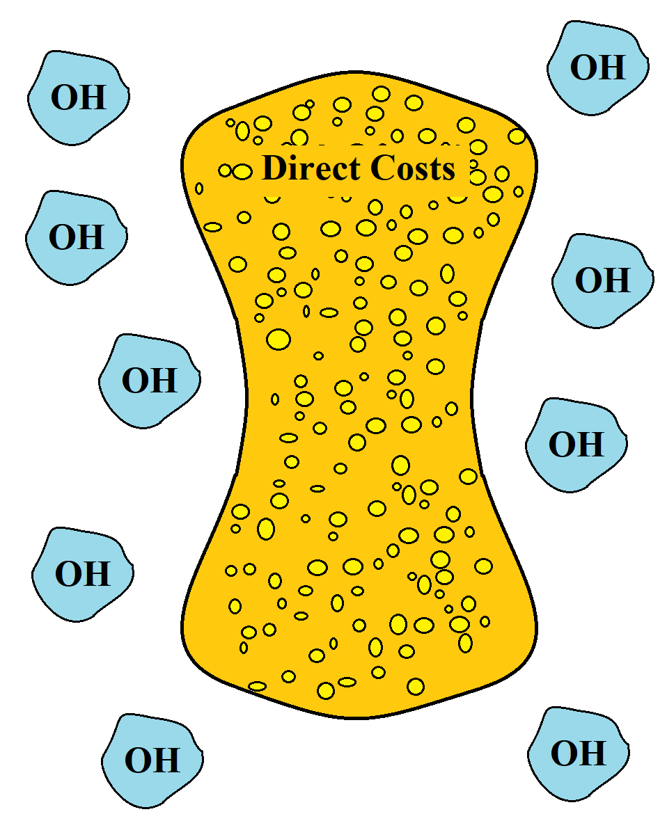
So, firms traditionally have allocated or applied overhead costs (those two words mean the same thing in this context). That means they create some fictional but presumably reasonable estimate for how much overhead should belong to each unit. This is called absorption costing because individual product units are located close enough to overhead costs that we make them absorb these costs like a sponge that is next to a kitchen spill.
Here’s an animation I made to show that. The sponge is an individual product unit. I’ve already traced certain direct costs to it. Then it absorbs some of the overhead floating around it. I act as if it has incurred those costs as well (even though I really don’t know which of the overhead costs traced to this product line, if any, belong to this product unit). Note that I abbreviate overhead as OH. That is very common. Also sometimes it’s abbreviated MOH for manufacturing overhead.
Deciding how much overhead each unit absorbs would be easy if all product units were always exactly alike. The firm should be able to just divide overhead costs evenly between units. (Actually, that’s more or less what we do in process costing, in Chapter 6, but we do run into some complications along the way.) If the firm has $1,000 in overhead costs and produces 200 units this month, each unit gets $5 in overhead cost allocated to it ($1,000/200 units).
However, many firms do not have products like that. Many firms customize individual products units—at least a little—for each customer. This is how the type of costing I’m covering this chapter, Job-Order Costing, gets its name. Each customized product unit is a “job” that is “ordered” with special features, leading to presumably different levels of overhead consumption or different product units. Job-Order Costing is often treated as the baseline method for traditional absorption costing.
For example, let’s say the 200 units produced this month are custom-ordered cars. These cars might differ considerably. One might have a sophisticated on-board computer that requires a lot of time on special equipment to program, set up, and calibrate. Another car might have a more basic computer system that requires only a small amount of time on this special equipment.
This special equipment is probably overhead (i.e. it’s not realistic to trace its costs directly to individual product units, but the firm knows it is incurring this cost because of a particular product line: custom cars). But just dividing this overhead cost evenly across both cars misrepresents which car is more responsible for the cost incurred by this special piece of equipment.
4.3.2 Cost Drivers and Pre-Determined Overhead Rates
4.3.2.1 Equations for Job-Order Costing
So Job-Order Costing assigns a cost driver, which is something the firm can trace to individual product units. Direct labor hours, direct labor cost (in dollars), machine hours, miles
The firm just piggy-backs overhead allocation—i.e. overhead absorption—onto the cost driver it’s already tracing to individual product units, assuming it is a good enough approximation of which products caused the overhead charge. The firm already has to trace direct labor hours and cost to product units. The firm might already trace machine hours or miles driven to individual product units as a quality control. Now it is also tracing these measures as cost driver for overhead costs.
How does a firm do this? The traditional technique is to estimate the numerical relationship between the cost driver and overhead before the period starts and then apply that overhead to product units as the firm traces actual cost driver consumption to those individual product units. This technique then, relies on a pre-determined overhead rate, or PDOH rate.
$$\Large PDOH\ Rate= \frac{Budgeted\ Overhead}{Budgeted\ Cost\ Driver}$$For emphasis, I want to re-iterate that the word budgeted is on both sides of that fraction. This rate is pre-determined, meaning it’s calculated using budgeted numbers before the period starts. Traditionally, at least, the rate does not change throughout the period.
Here’s an example.
Say a firm produces custom cars. Managers at the firm create a budget, in which they indicate that the firm will produce 200 cars next year. This budget for next year is finalized at the beginning of Q4 this year. On the same budget the firm also projects $5 million in overhead costs for next year. The firm can choose two different cost drivers: direct labor hours or machine hours. Last year the firm used direct labor hours. This year management believes it makes more sense to use machine hours since more and more of the overhead cost is due to sophisticated machinery. Budgeted machine hours for next year is 50,000. We already have enough to calculate the PDOH rate for next year, before that year has even started.
The PDOH rate is $100 per machine hour ($5,000,000 / 50,000 machine hours = $100 per machine hour).
As the firm starts producing cars, it applies overhead costs to individual product units using this rate of $100 per machine hour. If Car #125 uses 200 machine hours, it gets $20,000 in overhead costs applied to it. If Car #205 uses only 10 machine hours, it gets $1,000 in overhead costs.
$$\Large Applied\ Overhead = (PDOH\ Rate)(Actual\ Cost\ Driver\ Consumption)$$The amount of overhead applied to each car is the PDOH rate multiplied by the actual amount of cost driver consumption that is traced to that car. That is the moment when overhead costs floating around a product line get absorbed by an individual product unit.
4.3.2.2 The Cost Function in Absorption Costing
To put this into mathematical terms, I can rephrase the equation for π as follows. This restatement of the equation acknowledges that costs are driven by these different cost locations the firm recognizes.
$$\Large \pi_i = R(\cdot)-C(DM,\ DL,\ PDOH\ Rate,\ Actual\ Cost\ Driver)$$I’m not algebraically manipulating this equation like the equations in Chapter 3. That’s okay. Refining the cost function based on the cost’s location (including overhead absorption) serves a different purpose.
Like I said in Chapter 1, managers try to maximize long-term profit by tracing costs to the responsible product units, product lines, employees, teams, departments, etc. Look at the “i” subscript for π. I put that there to suggest this is not company-wide profit, instead it’s the profit for this sub-unit of the firm: e.g. this product unit, this product line, this employee, this team, or this department.
Tracing the profit of these sub-units is done to maximize the profit of the overall firm in the long-term. If a manager cannot evaluate the profitability of a sub-unit, he or she will have a hard time maximizing firm profit because he or she cannot see which sub-units of the firm are contributing a lot to firm profit and which sub-units are contributing little.
Look at the cost function, though. Overhead absorption is a driver of that function: PDOH rate and actual cost driver are variables driving the output of that function. Overhead absorption, then, drives the costs that sub-units of the firm are held responsible for. Inaccurate absorption of overhead costs can create some problems because it can make profitable sub-units look unprofitable and vice versa. I discuss this in the future chapters.
4.3.3 Inventory Accounts and Overhead Control
For a manufacturing firm, there are three inventory accounts: raw materials inventory, work-in-process inventory, and finished goods inventory. Also important for manufacturing firms: the cost of goods sold account and the overhead control account.
The raw materials inventory account (or RM) simply shows the dollar value cost of raw materials that have been purchased but that are still waiting in the warehouse waiting to be used in production.
The work-in-process inventory account (or WIP) simply shows the dollar value cost of inputs—raw materials, labor—that have been used in production on the floor of the factory. It also reflects the overhead that has been applied to those units in production on the factory floor.
The finished goods inventory account (or FG) simply shows the dollar value cost of products that are finished, have left the factory, and are now waiting for sale in the storeroom or distribution center, depending on the firm.
The cost of goods sold account (or COGS) is an expense account that reflects the dollar value cost of the products sold from the storeroom (or distribution center).
The overhead control account (or OH control) is a special expense account. On its debit side it shows overhead costs actually incurred. On its credit side it shows overhead costs allocated to WIP (using the PDOH rate/cost driver rationale explained above).
So when I say the overhead cost is applied, I mean it gets credited OH control and debited to WIP. That happens as quickly as actual cost driver consumption is traced to individual product units in WIP. Here’s the entry for Car #125 from the example above.
Dr. WIP (Car #125) 20,000
Cr. OH Control 20,000
Obviously this cost is coded for the specific WIP sub-account for the product unit in question so that unit can be held accountable for the overhead cost that the firm thinks the unit is responsible for (that’s the whole point!). For my purposes, though, I will treat WIP as a single account rather than a set of subsidiary accounts that distinguish between the cost for each car in WIP.
The process of allocating overhead to WIP based on tracing actual cost driver consumption is repeated until the end of the month.
4.3.4 Closing the OH Control Account
At the beginning of every month, accounting departments in every nation do their part to save the world. They do this by closing out last month’s income statement accounts. No one yet knows the havoc it would wreak on an unsuspecting planet to leave one of these accounts with a non-zero balance.
I need to sit down just thinking about it. It could be worse than dividing by zero.
OH control is an expense account. Closing it out is a little weird, though, because it does not have a reliable debit balance like most expense accounts. Yes, when an overhead cost is incurred, it gets debited. Like this.
Dr. OH control 50,000
Cr. A/P (maintenance contractors) 50,000
Dr. OH control 120,000
Cr. Wages payable (supervisor salary) 120,000
Dr. OH control 1,000
Cr. Shop supplies (per physical count) 1,000
Dr. OH control 70,000
Cr. Utilities payable (electricity and gas) 70,000
But it is also getting credited every time we trace cost driver consumption to a product unit.
Dr. WIP (Car #125) 20,000
Cr. OH Control 20,000
Dr. WIP (Car #205) 1,000
Cr. OH Control 1,000
Dr. WIP (Car #27) 100,000
Cr. OH Control 100,000
Dr. WIP (Car #56) 121,000
Cr. OH Control 121,000
Guess what! Cost driver consumption, which causes a debit to this account, doesn’t line up with overhead costs being incurred, which causes a credit to this account. This account could have a credit or a debit balance at the end of the month. For example, in the example above, the OH account will look like this in the trial balance.
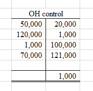
If it has a credit balance at the end of the month, like in this example, they say the firm overapplied overhead. The firm is said to have underapplied overhead if it has a debit balance at the end of the month. This makes a lot of sense. If there’s a credit balance, then our PDOH rate led us to apply more overhead dollars to individual product units than we actually incurred. If there’s a debit balance, then our PDOH rate led us to apply fewer overhead dollars to individual product units than we actually incurred.
The entry to close this account (and save the world!) could be either a credit to OH control or a debit to OH control. But where are we closing the account out to? What’s the other half of this entry? Tell us, tell us, TELL US!
You have two options.
- Close it out to COGS.
- Close it out to WIP, FG, and COGS (ratably, based on product units in each account)
Firms often just close the account out to COGS, effectively ignoring it, especially when the amount is relatively small.
If the amount being closed out is relatively large, though, firms want to make sure some of that entry goes to inventory accounts. Otherwise the units still on the factory floor (WIP) or on the showroom floor (FG) have inappropriately high or low allocations of overhead. That makes next period’s cost numbers inaccurate when those product units are eventually sold and their inventory value moves to COGS.
4.3.5 Job-Order Costing
Below I have an animation that walks through a general example of inventory accounts. When this example gets to closing the OH control account, I use the more complex method: closing it out to COGS, FG, and WIP.
Here are three useful terms and their position in this example. I’m sure this is review for you.
Cost of Goods Manufactured, or COGM, is captured in the movement of cost from WIP to FG, which makes sense because when products become finished goods they have been “finished”—or, “manufactured“. This is shown in Entry #6.
Cost of Goods Available for Sale, or COGAS, is cost of goods manufactured plus the beginning finished goods balance. It represents the costs of product units that were available for sale during the period. Because I have no beginning balances in this example, cost of goods available for sale and cost of goods manufactured are the same.
Cost of Goods Sold, or COGS, is a well-known account. The cost of product sold is indicated by the movement of costs from FG to COGS (which might seem obvious, but I think it’s worth pointing out), as well as the movement of underapplied OH costs to COGS as the firm closes out the OH control account. Thus COGS goes up and down in Entry #7 and Entry #8.
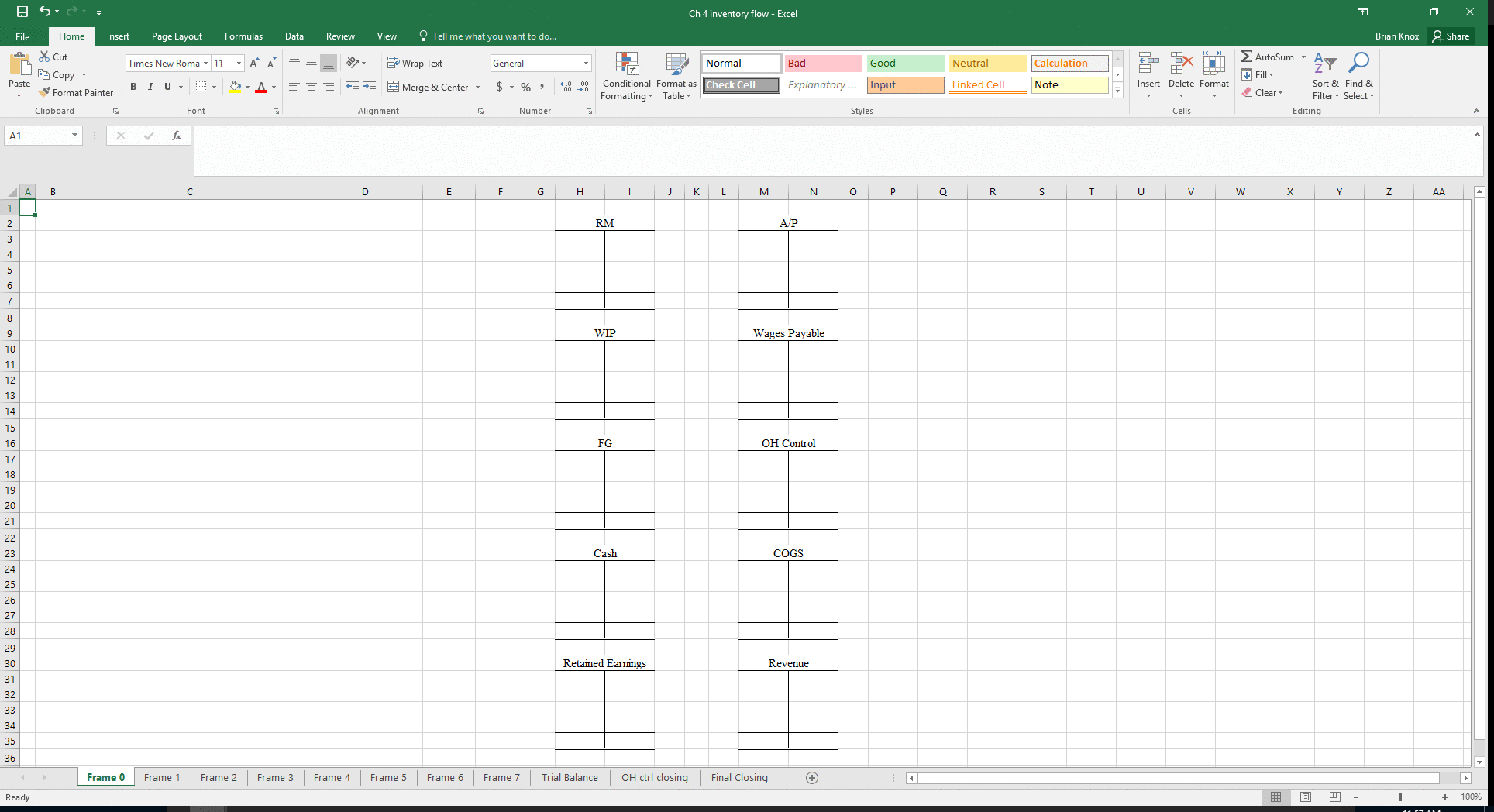
I’ll point out that Entries #6 and #7 reference job-order data. I’m providing that information in this example. It is not something you could have teased out from the previous entries. It is just the amounts observed and traced by the company.
4.4 Department PDOH Rates
4.4.1 Heterogeneous Department Overhead
Does the whole firm use the same PDOH rate? It depends on how heterogeneous the firm’s departments are. Assuming products pass through multiple departments in the manufacturing process and each department has its own budget for overhead cost and cost driver consumption, then each department could develop its own PDOH rate.
It could be worthwhile to do that if different departments tend to generate significantly distinct types of overhead. These different types of overhead might call for different cost drivers and thus different PDOH rates.
Using the custom car example, let’s assume there are multiple stages of custom car production: a frame stage and an interior stage. Each stage is performed in a separate department. The frame department uses heavy machinery to assemble the frame and any mechanical components that are attached to the frame. The interior department uses manual labor to create the unique look of the car’s interior.
The overhead in the frame department is mostly from the machinery that department uses, whereas the overhead in the interior department is mostly from the salaries of supervisors who oversee assembly line workers (who in turn supply “direct labor” that the firm traces to individual product units).
What should the company use as a cost driver? Machine hours? That makes sense for the frame department because the machine hours spent on each product unit probably does a decent job of approximating the overhead cost that belongs with each product unit.
But do machine hours do a good job of approximating overhead in the interior department? Probably not. Supervisors’ time spent on a product unit is less likely to be related to the machine hours spent on a product unit. Direct labor hours is probably a better cost driver.
This firm would likely be a good candidate for department PDOH rates: one rate based on machine hours in the frame department and a one rate based on DL hours in the interior department.
This kind of profit equation gets more complicated. The subscripts in the equation below show which department the PDOH rate is for.
$$ \pi_i = R(\cdot) – C(DM,\ DL,\ PDOH\ Rate_1,\ Actual\ Cost\ Driver_1,\ PDOH\ Rate_2,\ Actual\ Cost\ Driver_2)$$4.4.2 Heterogeneous Product Overhead
Heterogeneity is not just a question of department-to-department differences in overhead costs. What about significantly distinct products that consume significant distinct types of overhead as they go through the same department? Two products might be different enough in how what type of a department’s overhead they use that the PDOH rate procedure I’ve outline in this chapter creates very inaccurate estimates of product cost.
Chapter 5 details a procedure that attempts to address this.