Chapter 7 Guided Practice Problems
7.1 Variance Analysis Theory
7.1.1 Variance
One of the purposes of cost accounting is to hold people and things responsible for the costs they cause. Variance analysis plays a key role in this, but it goes deeper than I discussed in earlier chapters.
Since Chapter 2 I’ve repeated the idea that managers can better maximize long-term profitability if they know the profitability of different product units, product lines, departments, teams, regions, and/or individuals. Again, managers want to hold people and things responsible for the costs they cause because then managers can choose to have more of whatever is profitable and less of whatever is unprofitable in future periods.
This chapter (along with Chapter 9) adds a critical layer to this. Variance analysis does two things at once: (1) it narrows down responsibility for costs in a quasi-scientific manner, and (2) it suggests what action managers might take to increase future-period profit.
Variance analysis: the comparison of actual results against expectations in such a way that it suggests a specific action.
Variance: The difference between budgeted results and actual results.
Variances are usually expressed as absolute values followed by either “unfavorable” or “favorable,” based on whether the variance pushes firm profit lower or higher, respectively.
Rule of Thumb for Variance Analysis: If the difference between an actual and budgeted result (i.e. actual less budgeted) is negative difference, then that’s either an unfavorable revenue variance or a favorable cost variance. If the difference is positive, then that’s either a favorable sales variance and an unfavorable cost variance.
7.1.2 Total Budget Variance
The simplest variance is the difference between what was budgeted to happen and what actually happened. This is sometimes called total budget variance.
You can calculate the total budget variance for revenue, cost, or profit.
7.1.3 The Profit Equation and Variance Analysis
If variance is the difference between budgeted results and actual results, then I can restate the profit equation as follows.

Actual profit is driven by (1) budgeted revenue and cost and (2) variances. This might seem small, but it dramatically changes how we measure costs and profits (I discuss this a little more in Sections 7.7).
This setup also implies a relationship across time. The firm developed the budget last period, but actual numbers are from this period. Variances link the two periods. Furthermore, variances help inform the firm’s budgeted numbers this period, including actions the firm takes to improve actual profit next period.
As I’ll discuss in Chapter 9, the budget is a vehicle for knowledge. Theoretically, it represents the firm’s collective knowledge about itself: how it makes money and how it spends money. Understanding where that self-knowledge falls short (i.e. where variances arise) helps the firm learn more and more. A firm that understands itself is one that can truly maximize profit.
This is why I claim variance analysis is a quasi-scientific activity: it helps build the firm’s knowledge about its past, present, and future.
7.1.4 Quasi-scientific Responsibility Assignment
The scientific method is a rational set of activities designed to allow a person (or group of people) to test what he or she believes and expects, thereby allowing new knowledge to be gained, based on the most informative evidence available.
The scientific method, in abbreviated form, looks like this.
- Develop a hypothesis (i.e. an expectation) from prior observations or experience.
- Check if reality supports your hypothesis through a controlled experiment or careful analysis of extant data.
- Revise expectations as necessary based on results from Step 2. Return to Step 1.
This pattern closely resembles the budgeting, costing, and variance analysis pattern followed by most modern firms of significant size.
- Develop a budget (i.e. an expectation) from prior observations or experience.
- Collect data (especially cost data) during the period and carefully trace it to sub-components of the firm identified through the budget.
- Revise expectations as necessary based on results from Step 2. Return to Step 1.
Variance analysis helps the firm (in Step 2) trace actual costs to responsible sub-components of the firm and leads to revised expectations (in Step 3).
To be fair, this pattern of budgeting, costing, and variance analysis is somewhat unlike the scientific method because it is not performed independently and doesn’t usually involve widely publishing rich theories to increase humankind’s knowledge. So I don’t think it’s fair to call this process a truly “scientific” process.
But the similarities are strong enough that I feel justified calling it quasi-scientific. Managers do develop, effectively, a quasi-scientific theory of the firm: why it makes money, why it spends money, where it is most profitable, where it is least profitable. Managers might not publish their theory to increase human knowledge, but they do formalize it through a budget and use it to increase future-period profit.
The most important similarity, for my purposes anyway, is that this pattern involves developing an expectation and comparing actual results against that expectation in a controlled and careful way. If you understand that, you will have a much more complete understanding of variance analysis.
7.1.5 Variance Analysis Suggests Action
Comparing actual results against budgeted results seems very simple. Just subtract one from the other, right?
It’s not that simple. Managers only invest time and money in variance analysis because it will help them improve future-period profit. That means the comparison between budgeted results and actual results has to be done in a way that suggests at least one action that can be taken to improve profits in the future.
But total budget variance, the only variance I’ve introduced thus far, could be caused by hundreds, thousands, even millions of things. Managers are hardly any closer to knowing how to improve profits simply by knowing total budget variance.
Variance analysis, to be successful, has to subdivide variances in such a way that each variance figure identifies a course of action that would repeat the variance next period (if favorable) or avoid it (if unfavorable).
This is largely what I mean when I say variance analysis compares budgeted and actual results in a “controlled and careful way.” If there are lots of possible causes for a variance, how can I decide which cause to single out for action? I have to control for other causes first, and only look at how much variance is realistically due to a particular cause. That involves subdividing variances based on their cause, and it’s a prerequisite for actionable information.
A lot of the headache for students comes from having to subdivide variance into actionable chunks of information. But it’s also a critical component of variance analysis, without which the whole procedure would probably be worthless. So suck it up, buttercup!
7.1.6 Standards: Price and Quantity
The key to subdividing variances is “standards.”
But standards are simply mini-expectations that, when combined, lead us to budgeted total dollar amounts. If, for example, a firm expects direct labor wages to be $10 per hour, then $10 per hour is the standard price for direct labor. Then if the firm expects each unit to take 2 direct labor hours, the standard quantity per unit is 2 direct labor hours.
See how this works? The standard prices and quantities are the building blocks that go into making a budget. In the example above if the firm expects to make 1,000 units, it would budget direct labor cost of $20,000 (i.e. 1,000 units * 2 direct labor hours per unit * $10 per hour).
If a firm is going to subdivide variances from a budget into actionable chucks of information, then it has to use the building blocks that were used to develop the budget in the first place.
Continuing with the example let’s say actual direct labor costs were $25,000. The firm could calculate the direct labor variance as an unfavorable variance of $5,000, but that doesn’t help much because that information doesn’t lead to an action. Is that $5,000 unfavorable variance due to higher direct labor prices? Is it due to higher unit sales? Is it due to the more direct labor hours required per unit? If the firm knew which standard used to build the budget had fallen short, it would suggest an action.
Rule of Thumb for Variance Analysis: If you want a variance to be actionable, your variance should be the difference between two numbers that differ by only one standard-versus-actual attribute.
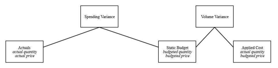
Here’s the basic shape of variances (I’ll explain more on each piece of this diagram later).
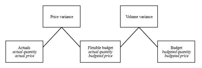
At one end of the spectrum, you have actual figures. At the other end, you have the budgeted figures. (The difference between these two extremes is the total budget variance.)
Variance analysis moves incrementally from one extreme to the other, comparing just one standard-versus-actual result at a time. This leads to variances that tell you how much of total budget variance is due to each cause.
7.2 Revenue Variances
7.2.1 General Causes of Revenue Variances
Let’s start with revenue variances. Here’s the key question for revenue variances: why would
- There might be a variance in the price units were sold for.
- There might be a variance in the volume of units that were sold.
7.2.2 Sales Price Variance
Did the firm sell a product for a higher or lower average price than it budgeted? Sales price variance measures that difference by comparing what budgeted revenue would have been if the firm knew how much actual revenue.

When I rearrange this equation algebraically, I arrive that the following.

Sales price variance is actionable, but the action it suggests will depend on the firm’s strategy. A cost leadership firm might actually prefer an unfavorable variance here, which could mean the firm is pushing prices lower and lower to undercut competitors. (In other words, this kind of firm presumes that unfavorable price variances are offset by favorable volume variances.)
A favorable price variance for a firm with a differentiation strategy, on the other hand, suggests customers may increasing perceive the product to be
With a little investigation the firm could use this variance to develop a plan to improve profits next period.
7.2.3 Sales Volume Variance
Did the firm sell a higher or lower number of units than it budgeted? Sales volume variance measures that difference by comparing budgeted revenue with what budgeted revenue would have been if the firm knew how many units it was going to sell (all at the budgeted sales price)

When I rearrange this equation algebraically, I arrive that the following.

Sales volume variance is actionable because it reflects the overall volume of sales. An unfavorable sales volume variance could reflect an unmotivated sales force, poor brand recognition, lack of consumer confidence, or competitive pressure.
With a little investigation the firm could use this variance to develop a plan to improve profits next period.
7.2.4 Quick Note on Multi-product Firms’ Sales Volume Variance
These two revenue variances (i.e. sales price variance and sales volume variance) are usually all you need in a single-product firm. In a multi-product firm, you might need a little more. That’s because multi-product firms’ sales volume variances could reflect overall sales changes or just a change in the sales mix. These two causes would suggest different actions. Thus sales volume variance might not be actionable enough on its own for a multi-product firm.
So multi-product firms often break down sales volume variance into sales mix and yield variances. I cover this later in Section 7.8 because mix and yield variances are relevant to cost variances as well.
7.3 Cost Variances
7.3.1 Cost Variances and Flexible Budgets
Firms are also interested in whether costs match expectations. Product costs, such as direct labor and direct materials are among the most important of these cost variances.
Direct labor and direct material variances largely follow the same pattern demonstrated by the revenue price and quantity variances.

But there are some key differences.
The first question: what is “budgeted quantity”? The firm formed the budget last period. As part of creating that budget, the firm estimated how many units it would produce and then estimated how many direct labor hours and units of direct materials it would need to reach that level of production.
That estimation of production was almost certainly wrong. So some of the difference between budgeted and actual cost numbers is because the firm actually produced a different number of units than budgeted. Production volume is a possible cause of quantity variance.
It’s important to separate out production volume as a cause of direct labor and direct materials quantity variances. Otherwise, the firm could not come up with an actionable variance.
For example, last period I budgeted 100 units of production for this period. The standard quantity for direct labor is 0.5 direct labor hours per unit produced. Therefore, I budgeted 50 direct labor hours. Actual numbers come back: 110 units produced and 60 direct labor hours.
Direct labor hours varied by 10 direct labor hours: 60 actual hours versus the 50 budgeted hours. What action does this variance suggest? It’s unclear. At least some of those extra direct labor hours were caused by the 10 extra units produced. It’s obvious that when more units are produced, more direct labor hours are required. Some of those additional direct labor hours are probably good news: the product is more popular than I thought.
But, on the other hand, some of those additional direct labor hours could also be due to inefficiency. Some of those extra hours could be from my workers watching Netflix at work instead of working. That’s bad news.
To solve this the budgeted quantity for quantity variances needs to be drawn from a flexible budget, which is what the budget from last period would have looked like if the firm knew, back then, what actual production was going to be.
Static budget: A budget based on last period’s budget for this period’s volume.
Flexible Budget: A budget based on this period’s actual volume (while still using all other assumptions as the static budget).
A static budget (column F) and a flexible budget (column G) are both shown below. For the flexible budget, I used the same assumptions as the static budget but changed the volume to 110 units (compare cells F3 and G3).
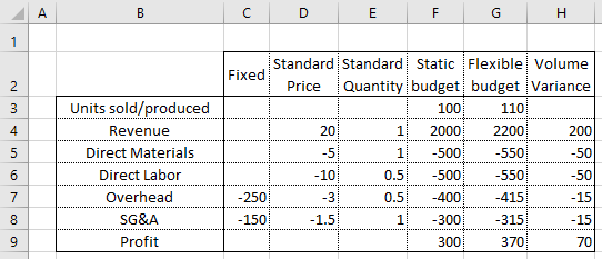
By taking budgeted quantity numbers from the flexible budget instead of the static budget, I can isolate and remove some variance that is just due to the difference in production volume (i.e. the “volume variance” figure in the far-right column).
Rule of Thumb for Variance Analysis: For cost variances, “budgeted quantity” is always drawn from the flexible budget, not the static budget. That is, it’s what the budgeted amount of the cost input would have been if the firm knew in advance what actual production volume would be.
So the diagram above better shown as follows, at least for cost variances. (The asterisk reflects how the flexible budget’s “budgeted quantity” is how much input would have been budgeted at the actual number of units produced).
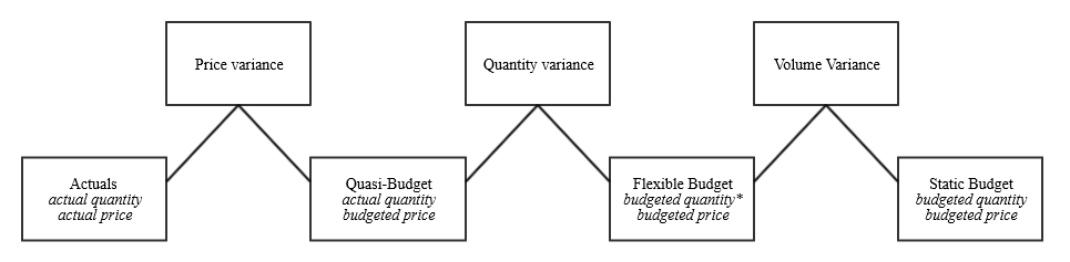
Here on the cost variance side, I focus on the price and quantity variances. This is where the most actionable information tends to be. In the below discussion, I usually ignore volume variance and start with flexible budget numbers
7.3.2 Helpful Hints
Also notice that, for the above revenue calculations, quantity was expressed as a total figure and price was expressed per unit.
This is an important pattern that continues with cost variances.
Contrast this to standards for cost variances, which as I say below are always per unit numbers. Standard quantity is the quantity of an input (direct labor, direct materials, or overhead) per unit produced. Just because that’s the standard quantity doesn’t mean you can plug that number in for actual or budgeted quantity.
Rule of Thumb for Variance Analysis: When working the equations for variances, quantities are expressed as totals (e.g. actual totals or budgeted totals at the standard quantity), while prices are expressed per unit.
7.4 Direct Labor Variances
7.4.1 Direct Labor Quantity Variance
As long as you remember that budgeted quantities refer to the flexible budget, direct labor variances can be calculated in a way that is very similar to revenue variances.
First, there is the direct labor quantity variance. Sometimes this is called an “efficiency” variance.

Rearranged, I get the following.

An unfavorable quantity variance suggests the firm is spending more time than budgeted on each unit produced. This might be due to poor training, poor retention (which lowers the average tenure and skill level of each employee), or excessive re-work due to low quality materials. With a little investigation a plan of action can be easily developed from this variance.
7.4.2 Direct Labor Price Variance
Second, there is the direct labor price variance. Sometimes this is called a “rate” variance.

Rearranged, I get the following.

Labor rate often become unfavorable when too few workers are employed (meaning overtime pay), more highly skilled worker time was required than budgeted, and benefits are higher than budgeted. With a little investigation this is actionable information.
7.4.3 Direct Labor Variance Journal Entry
How does a firm record these variances? Many firms build these variances into several T-accounts, each bearing the name of the variance they represent. These T-accounts are debited or credited as costs are applied to WIP.
Here’s the basic idea. Let’s say the flexible budget, at 4,000 units of production, budgets $8,000 for direct labor. Standard price is $8 per direct labor hour and standard quantity is 0.25 hours per unit.
Actual direct labor costs are $11,500. This $11,500 has to be recorded at actual cost of $11,500 in the wages expense account. The FASB frowns on firms not recording expense accounts at actual values (as in, they can send you to prison).
This expense gets transferred to WIP because it reflects direct labor cost, which is a product cost and needs to inventoried.
But if the firm uses the full standard costing system, that means it records all inputs to WIP at standard cost: debiting WIP for $8,000 of direct labor cost. Now the journal entry is unbalanced (i.e. Dr. WIP $8,000 and Cr. Wages Expense $11,500).
This journal entry is balanced by debits to the variance accounts “Direct Labor Quantity Variance” and “Direct Labor Price Variance.”
Let’s say that actual quantity of direct labor hours was 1,250 (or 0.3125 per unit) and the actual price was $9.20 per direct labor hour. Then the variances would be as follows.
Direct Labor Quantity Variance: $10,000 (budgeted price of $8 multiplied by actual hours of 1,250) – $8,000 (budgeted price of $8 multiplied by budgeted hours of 1,000) = $2,000 direct labor quantity variance.
Direct Labor Price Variance: $11,500 (actual price of $9.20 multiplied by actual hours of 1,250) – $10,000 (budgeted price of $8 multiplied by actual hours of 1,250) = $1,500 direct labor price variance.
In the spreadsheet below I show the journal entries related to direct labor in a full standard costing system. Entry #1 is entered when wages are incurred. Entry #2 is entered when direct labor hours are traced to product units. (These two events might be at the same time.)
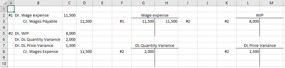
Rule of Thumb for Variance Analysis: In the full version of standard costing that this textbook covers, costs debited to WIP are always at standard. Costs debited to expense accounts (not including variance accounts) are always at actual. The difference between standard cost and actual cost goes to one or more variance account.
Rule of Thumb for Variance Analysis: Cost variance accounts are expenses. Debits to these accounts are for unfavorable variances. Credits to these accounts are for favorable variances.
7.5 Direct Materials Variances
7.5.1 Differences Between Direct Materials and Direct Labor
Direct materials variances use the same names as direct labor variances. But there’s a big difference. Specifically, direct materials quantity variances and direct materials price variances use different definitions for “actual quantity.”
Direct materials price variance defines actual quantity as the actual quantity purchased. Direct materials quantity variance defines actual quantity as the actual quantity used.
(Firm’s don’t have to do this. Some don’t. But it does a far better job of assigning responsibility, assuming there are separate purchasing and operations departments and/or managers.)
The reason for the difference is that direct materials price is determined when direct materials are purchased. The responsible parties are purchasing manager or the purchasing department in general. How much direct material is used is determined when direct materials are added to work in process. The responsible party in this case is the factory manager or factory workers in general. By using two different actual quantities, direct materials variances better assign responsibility.
This wasn’t a problem with direct labor because it’s a relatively perishable input. Materials can be saved in the warehouse for next period if not used right away, and direct materials purchased is usually different from what is used. It’s not possible (or legal in most states) to buy labor and store it in a warehouse until next period. Direct labor purchased is the same as direct labor used as far as this textbook is concerned.
If you can remember that actual quantity will be different for quantity and price variances, you can calculate direct materials variances in a way that is very similar to direct labor variances.
7.5.2 Direct Materials Quantity Variance
Just like direct labor, the direct materials quantity variance measures the difference between flexible budget direct materials cost (i.e. at actual volume of production) and what flexible budget direct materials cost would be if the firm knew how much direct materials it would use.


This is also sometimes called an “efficiency” variance or a “usage” variance. An unfavorable direct materials quantity variance suggests the firm is being inefficient with its direct materials on the production floor. Perhaps this is due to poor quality materials. Perhaps this is due to unskilled workers. Perhaps this is due to wasteful machinery or processes. With a little investigative effort, the firm can figure out an action to improve this variance.
7.5.3 Direct Materials Price Variance
Just like direct labor, the direct materials price variance measures the difference between actual direct materials cost and what flexible budget direct materials cost would be if the firm knew how much direct materials it would use.


An unfavorable price variance suggests a problem within the purchasing department of the firm or a change in the external market for this input. It could also be related to the firm’s differentiation strategy and purchasing high-quality direct materials. With a little investigative effort, the firm can develop an action plan to improve this variance.
7.5.4 Direct Materials Variance Journal Entries
7.5.4.1 Unique Considerations for Direct Materials Variance Journal Entries
There are separate entries for direct materials variances. That’s for two reasons. First, the two variances are typically realized at two different times: the time of direct material purchase and the time of direct material use. So it makes sense to record each variance when the cost is incurred.
Second, the two variances, added together, do not always equal the total difference between actual cost and flexible budget cost, since actual quantity purchased is usually different from actual quantity used.
When students hear this they inevitably ask me where the rest of the difference went. This is a reasonable question. The difference is sitting in the warehouse, waiting to be put into production. Let me explain.
If actual units purchased and actual units used are different, it implies a change in the number of direct materials in the warehouse. Any gap or overlap between the two direct materials variances reflects the value of direct materials stored in or removed from the warehouse, i.e. the direct materials inventory account.
7.5.4.2 The Direct Materials Price Variance Account
The firm can record the price variance as part of its entry recording purchase of new direct materials. The credit will be the actual cost, usually credited to either cash or accounts payable.
The debit to direct materials will be at standard price. One of the rules of thumb for variance analysis is that WIP receives all costs at standard. The direct materials account serves as a half-way home for these costs. They’re not fully at standard, since they still reflect the actual quantity of direct materials units purchased. But they are halfway there.
This leads to an uneven journal entry. To balance it, the firm debits or credits the difference to the direct materials price variance account.
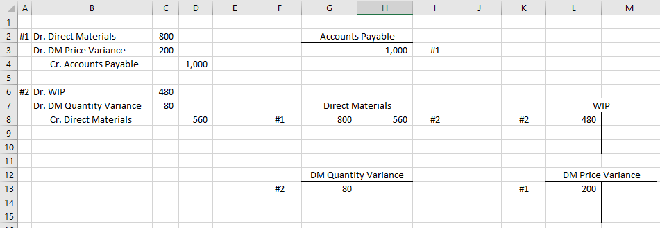
For example, assume the firm purchases 10 ounces of a rare earth metal for $100 per ounce. The standard price for this direct material is only $80 per ounce. Therefore actual cost is $1,000 and the debit to direct materials is $800. The $200 difference has to be a debit to the direct materials price variance account.
Dr. Direct Materials $800
Dr. DM Price Variance $200
Cr. Accounts Payable $1,000
7.5.4.3 The Direct Materials Quantity Variance Account
When units are moved from the warehouse (or wherever they’re kept) and put into production, your instinct may be to credit the direct materials account for the value of those units and debit the WIP account for the same amount.
If that’s your natural instinct, good. Let the cost flow through you.
And it’s almost right. But remember that WIP is always debited at standard: standard price and standard quantity. This means there will be another unbalanced journal entry.
The difference between the debit and the credit goes to the direct materials quantity variance account.
Returning to the above example, let’s say 7 ounces of rare earth metal are put into production this period, the journal entry will include a credit to direct materials of $560 (standard price of $80 times actual quantity used of seven).
Debit to WIP is based on full standard cost. Let’s say the standard quantity is actually 6 ounces, that is, given the number of finished goods units produced, the budget would predict that the company use six ounces. Debit to WIP is $480 (standard price of $80 times standard quantity used of 6).
The difference between the two goes to the direct materials quantity variance. That line of the journal entry is a debit, meaning the variance is unfavorable.
Dr. WIP $480
Dr. DM Quantity Variance $80
Cr. Direct Materials $560
7.6 Overhead Variances
7.6.1 Contextual Note
Among cost variances, I find overhead variances to be less useful than direct labor or direct materials variances. There are two reasons for this.
First, overhead absorption is a loose guess (i.e. a PDOH rate, activity-based costing scheme, equivalent units, etc.). That means there are likely to be confounding alternative causes of overhead variances, making them in turn less scientific.
Second, it is more likely that responsibility for overhead costs, even after additional investigation, is spread across several managers and/or departments. That means overhead variances are often less easily actionable than other cost variances.
Regardless, many companies calculate overhead variances and seem to get some good use out of them. One reason may be that overhead variances can offer confirming evidence of direct material or direct labor variances.
For example, if an unfavorable direct materials quantity variance suggests the firm is using sub-standard material, then a variable overhead variance is likely to be unfavorable as well (e.g. poor quality material likely increases maintenance costs for machinery). A favorable direct labor price variance and an unfavorable direct labor quantity variance sound a lot the firm cut corners and hired a low-skilled workforce. An unfavorable overhead variance (e.g. driven by a need for extra human resources costs or training costs) could help confirm this diagnosis.
7.6.2 Variable Overhead Variances
Overhead variance regimes typically separate variable overhead from fixed overhead. So they come up with separate variances for variable and fixed overhead. As if your life wasn’t hard enough.
When forming the budget, variable and fixed overhead are typically added together as total overhead cost. Then, in job-order costing systems, this total overhead cost is used as the numerator to compute a PDOH rate. That is, a PDOH rate usually includes both variable and fixed overhead costs.
So you usually cannot just use the PDOH rate as the standard price of overhead. You have to dig into the budget to find the variable overhead cost rate per unit of the cost driver. That is the standard price of variable overhead.
I will simply call this the PDVOH rate, to mean “predetermined variable overhead rate.” That is the standard price.
In a similar vein the standard quantity is the budgeted cost driver consumption per unit produced.
From there one can calculate variable overhead variances basically the same way as direct labor and direct materials variances.
Variable overhead quantity variances:


Variable overhead price variances:


Variable overhead variances mean something a little different than direct materials and direct labor variances.
The quantity variance reflects the variance due to how much cost driver the firm used. If there is a solid case that the cost driver is reliably causing variable overhead costs, then this could reflect the quantity of overhead consumed. However, oftentimes this relationship is loose. For example, does using more direct labor hours than budgeted really have a strong relationship to the maintenance costs for factory machinery?
If we assume the relationship is indeed cause-and-effect, then unfavorable variable overhead quantity variances suggest the firm was inefficient in its use of the cost driver (per unit produced), as expressed by the additional and excess variable overhead costs incurred as a result.
Variable overhead price variance reflects the dollar-to-cost-driver relationship between the cost driver and variable overhead costs. It is somewhat tautological. An unfavorable price variance suggests that the actual cost driver consumed cost more than was budgeted, i.e. that the firm paid more for some type of overhead than it should have.
Without knowing a sub-type of overhead cost that cost too much or the quality of the estimation that lead to the PDVOH rate in the first place, it is relatively hard to use this figure for evaluative purposes.
7.6.3 Fixed Overhead Variances
Fixed overhead variances are a little different. There is little sense in trying to parse out a price and quantity variances since the price of fixed costs per unit will vary based on the number of units produced (since fixed costs are, by definition, fixed).
Unlike other variances, the firm starts from what was applied to WIP via the PDOH rate (i.e. Applied Cost, as shown below). The firm compares that number against the static budget. The difference is often called the fixed overhead volume variance.
Since fixed costs, by definition, do not vary with volume, the static budget and the flexible budget are the same for fixed overhead costs. To avoid confusion I do not use the term flexible budget for this variance.
But the fixed overhead costs applied to product units might be different from what was budgeted simply because the firm has higher or lower volume and due to the the mechanics of absorption costing. Absorption costing tends to lump fixed and variable overhead costs into a rate that is allocated per cost driver unit regardless of the costs’ fixed or variable nature.
Then the company compares the static budget to actuals. This difference is often called the fixed overhead spending variance.
Here are the variances written out mathematically. These two equations use the term PDFOH rate, which means the “predetermined fixed overhead rate.” This term expresses the portion of the PDOH rate that applies fixed overhead costs to units. It is the PDOH rate minus the PDVOH rate.


Note: In the FOH Volume Variance, the term “Actual Cost Driver * PDFOH” is the same as “Applied Costs.” Sometimes fixed overhead variance problems provide applied costs and don’t make you calculate it.
This favorability works like prior favorability for two reasons. First, as with the prior costs, if the left-hand number is higher than the right-hand number, then it is an unfavorable variance (see the diagram above). The diagram above correctly shows the static budget’s fixed overhead cost as being more leftward (or less hypothetical) than the allocated fixed overhead cost. Allocated fixed overhead cost is more contrived than static budget fixed overhead cost because allocated fixed overhead cost is based on the consumption of the cost driver. And that cost driver (very likely) moves up and down as volume moves up and down. So the allocation of fixed overhead matches a variable cost pattern in that it varies with production volume. Thus the cost driver-allocated of fixed overhead figure is more fictitious than the static budget figure. That static budget knows better than to treat fixed overhead as if it were a variable cost. The logic from previous cost variances about how to judge favorability as we move from the more hypothetical number (i.e. more rightward) to the more actual number (i.e. more leftward) continues to work.
The second reason is capacity. Fixed costs are costs you incur regardless of volume. If you have a low allocated fixed cost figure, it likely means you underutilized the capacity you bought with a fixed cost, and that wasted capacity is unfavorable. Let’s say you budgeted and paid $100,000 for a factory lease. But you produced a very low volume with that factory, leading to very low consumption of the cost driver, leading to a very low allocated fixed overhead cost figure. That is an unfavorable thing. That amounts to wasting at least part of the factory’s productive capacity that you paid $100,000 for. Thus, it is also unfavorable from the perspective of unused capacity.
7.6.4 Overhead Variance Journal Entries
As discussed in Chapter 4, overhead may already be recorded at standard. That’s more or less what a predetermined overhead rate does.
Here’s a great illustration to review (it comes from a great free online management accounting resource: maaw.info). In Chapter 4, I laid out the “Normal Historical” system that (1) records (in WIP) direct materials and direct labor at actual cost (2) while using the Overhead Control account as a filter to record only a standard amount of overhead cost in WIP (per unit of cost driver consumed).
We said at the end of that discussion that the balance of the Overhead Control account could indicate that overhead had been overapplied (for a credit balance) or underapplied (for a debit balance). In the case of many, but not all, normal historical
Overapplied or underapplied overhead is basically the same as a favorable or unfavorable variance, it just isn’t broken up yet into the individual variable and fixed overhead variances. Now that we’re looking at the “Standard” paradigm (from the illustration above), all input costs are debited to WIP at standard and the remainder is partitioned out into the four variances, as calculated using the equations above.
It’s really as simple as that. (See MAAW’s illustration of the T-accounts the journal entries go to. “Factory Overhead” in this illustration is the same as the Overhead Control account).
7.7 Putting Together A Costing System
7.7.1 A Point on Terminology
When I introduced job-order costing in Chapter 4, I simultaneously introduced “normal costing” (from the illustration linked above) even without naming it as such.
There were two reasons for this.
First, it was important to focus on the idea of not recording actual overhead. That’s how a lot of firms do in practice. It is hard to create a job-order costing example without giving you some sense of how jobs might be assigned overhead costs that, by definition, aren’t being traced directly.
Second, I didn’t make the distinction between “normal costing” and other systems of costing because we weren’t covering those alternative systems. Now, in Chapter 7, we’re covering an alternative: recording all product costs at standard so we can extract variance information. In Chapter 8, we’ll cover another alternative: lean accounting uses only actual costs (called “pure historical costs” in the illustration I’ve linked to above) to avoid rewarding overproduction.
7.7.2 Standard Costing and Chapters 4, 5, and 6
Standard costing can technically be combined with any of the costing systems described in Chapters 4, 5, and 6. That’s because the “standard costs versus normal costs versus actual costs” decision answers a different question than the “job-order costing versus activity-based costing versus process costing” decision.
Here’s one more great illustration from MAAW. (You must click on that link or the rest of this subsection won’t make sense). Standard costing is an answer to the “Input Measurement Basis” question. That is, how do we measure WIP input costs: at actual or standard? You can record WIP at actual cost (i.e. “Pure Historical,” covered in Chapter 8), at standard (i.e. “Standard,” covered in this chapter), or at a mix of actual and standard (i.e. “Normal,” covered in Chapter 4).
Job-order costing and process costing, in contrast, are answers to the “Cost Accumulation Method” question. That is, job-order costing accumulates costs at the job-level and process costing accumulates costs at the process-level (or department-level). In a modern accounting system that means the computer effectively maintains separate WIP accounts for each job or for each process.
That illustration also lists “Hybrid” as an option. That means accumulating some costs at the job-level and some costs at the process-level (hybrid systems are sometimes called “operation costing”). Backflush cost accumulation is listed as well, which we’ll cover in Chapter 8.
Activity-based costing actually answers yet another question, “Inventory Valuation Method.” This is why I mentioned in Chapter 5 that you could technically build activity-based costing atop either a job-order costing system or a process costing system (although the latter is less common, in my view). The inventory valuation question determines which costs are considered inventory, an asset, and which costs are considered expense.
So, Chapter 4 and 6 were presented using the “Full Absorption” method, meaning all product costs (i.e. direct materials, direct labor, and overhead) were considered inventory costs. Full absorption is required for GAAP reporting. In Chapter 5, I said that ABC can include SG&A costs in inventory, and thus it is a departure from full absorption. We’ll cover what is considered an invetoriable cost under throughput accounting and direct costing in Chapter 8.
7.8 Mix and Yield Variances
7.8.1 Mix Variances
When multiple types of inputs go into a quantity variance, that variance is less useful.
- Revenue quantity variances, for example, might be affected by the mix of product 1 vs. product 2, product 1 premium vs. product 1 basic, product 2 brick-and-mortar sales vs. product 2 internet sales, etc.
- Direct labor quantity variances, for example, might be affected by the mix of high-skilled worker hours vs. low-skilled worker hours, permanent worker hours vs. contractor hours, regular hours vs. overtime hours, etc.
- Direct materials quantity variance, for example, might be affected by chemical 1 vs. chemical 2, ingredient 1 vs. ingredient 2, high-quality input 1 vs. low-quality input 1, etc,
In these situations, the quantity variance should be broken into mix and yield variances. A mix variance expresses variance due to differences the between the actual mix of substitutable inputs and the standard mix of those inputs.
You can think of the mix variance either as an equation or a table.

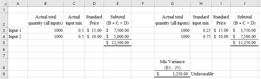
Both of these get you to the same place. The equation subtracts standard from actual first, then multiplies by standard price and sums across all inputs. The equation can provide you with a clearer picture of how the actual mix of inputs affected each input’s costs separately.
The table multiplies total input by mix percentage and standard price, then sums the actual costs and standard costs associated with these mixes separately. It can give you a clearer picture of why the overall variance is favorable or unfavorable. In this case, it is a $1,250 unfavorable variance because the actual mix included a higher percentage of the more-expensive Input 1 more than was expected.
7.8.2 Yield Variances
The yield variance reflects the variation between standard finished goods output (given inputs) and the actual finished goods output (given inputs).

Actual yield is the actual finished goods units completed.
Standard yield is the finished goods units you’d expect given total actual inputs at standard mix (i.e. standard total output / standard total input * total actual input).
Standard Price at Standard Mix is the standard input price for a single finished good unit (i.e. finished goods unit), assuming the inputs are at the standard mix and standard price (i.e. standard price of a batch of input units at standard mix / finished goods units per batch).
That might seem complicated, but it’s actually a familiar idea. It’s a lot like the plain old quantity variance you already know.
See, if you’re splitting the quantity variance into mix and yield variances, then there are multiple inputs that can be substituted for each other. Yield variance then is just the traditional quantity variance (i.e. how many finished goods units come from the given input units) adapted to this idea of substitutable inputs.
Here’s an example.
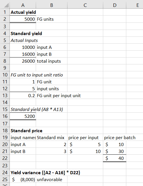
Let’s say a product requires two substitutable inputs, A and B. The standard mix is 2:3 (i.e. two units of input A for every three units of input B). For every 5 units of inputs A and B, a finished goods unit is typically produced. Standard prices are $5 for a unit of input A and $10 a unit of input B (actual prices are the same as standard prices).
Let’s say the firm used 10,000 units of input A and 16,000 units of input B and produced 5,000 finished goods units.
To find the yield variance, we need to calculate each of the three variables that go into the variance.
Actual yield is the 5,000 finished goods units actually completed. Standard yield requires calculation. Typically there is one finished goods units for every 5 input units. There are 26,000 input units (10,000 input A + 16,000 input B = 26,000 total input units), which should yield 5,200 finished goods units (using the terminology above: 1 standard output / 5 standard input * 26,000 actual input = 5,200). For simplicity, we’ll assume a batch is one finished goods unit, which takes 2 units of input A and 3 units of input B. That leads to a standard price of $40 (2 units of input A * $5 per unit of input A + 3 units of input B * $10 per input unit B = $10 + $30 = $40).
Then the yield variance is $8,000 unfavorable ([5,000 actual yield – 5,200 standard yield] * $40 standard price per output unit).