
Those volume problems, I can tame ’em.
Through CVP, they flee from me
‘Cause I provide the firm’s breakeven.
Chapter 3 Guided Practice Problems
3.1 Cost Characteristics: Cost Behavior
3.1.1 Special Kinds of Special Order Decisions
In each traditional decision from Chapter 2, you faced an either/or choice. You can make or buy. You can sell or process further. You can keep a product or drop it. You can accept a special order or reject it.
But special orders also had a “to be continued….” I hadn’t introduced critical terminology to understand special order decisions that aren’t either/or. Specifically, what if the special order doesn’t have a set price? What minimum price can a manager accept in negotiations for that special order? (I’ll call these “variable-price special order decisions” in Section 3.6)
For this style of special order decision, managers maximize profit by selecting the correct minimum price number out of an infinite set of numbers on the number line. This decision has an infinite number of alternatives. Even if I rounded to cents, attacking this decision with a table like profit maximization decisions from Chapter 2 would create an enormous table.
So managers instead define R(·) and C(·) in a way that allows them to algebraically solve for the optimal price floor out of an infinite set of numbers on the number line. The techniques in this chapter are astonishingly common. Managers are constantly using them to define firm profit and, especially, the C(·) function.
Compare the discussion in the rest of this chapter with my definition of a “decision” in Chapter 2. It actually fits pretty well.
3.1.2 The Algebra of Fixed and Variable Costs
Sometimes cost accounting classes downplay how much this part of the class leans on algebra. They try to phrase it all in real, practical terms. This is well-intentioned. But I think it’s ultimately better to face the truth: managers often define revenue and costs across a range of input variables, which means they’re using algebra. It makes more sense to have an algebraic equation for revenue and costs that
Algebra doesn’t just help with special order decisions. It also helps with decisions about volume, i.e. how many product units the firm should produce and
To solve volume problems, managers separate the cost function into variable costs and fixed costs. Variable costs are costs that are higher when the firm produces more units and lower when the firm produces fewer units. Fixed costs stay the same regardless of the number of units produced.
Managers typically identify variable and fixed costs by using statistical tools (like linear regression) or by using their professional judgment.
Because variable costs relate to the number of units produced, I can’t know what total variable costs are unless I know the number of units produced. So I express units produced with a variable, q, and multiply it by variable cost per unit, v. Fixed costs are always the same. I’ll express it as a separate variable, f. Since f doesn’t have a q next to it, I show that fixed costs do not vary based on volume. I end up with this equation, which looks like the prototypical algebraic expression of a line (y = mx + b).
$$\Large C(\cdot) = vq+f$$It’s important to remember that v represents variable cost per unit, while f represents total fixed costs. The term vq represents total variable costs.
Although revenues are less interesting in this regard, they obviously also increase with production (assuming the firm sells everything it produces). The sales price, p, makes the R(·) equation look like this.
$$\Large R(\cdot) = pq$$As promised in Chapter 1, more work was spent on the cost function than on the revenue function, since one must sort between variable and fixed costs to get C(·), whereas there’s only variable revenue in R(·).
3.1.3 All Step Costs and Curves
A little secret: both of these equations are a fiction that, at best, only approximate the actual cost and revenue functions. First, all costs in a firm are related to production: by step. Costs are flat for a certain range then step up when q gets high enough.
For variable costs and
For fixed
Usually, though, if I include a problem with a fixed cost, you can assume it won’t step up to the next level of fixed costs within the context of that particular problem (sometimes called the relevant range).
Second, v and p are not as stable as they seem. Prices are discounted all the time and can be dramatically affected by market changes. Variable costs per unit, v, can increase or decrease considerably as production fluctuates because of synergies, supply chain factors, and economies of scale.
But for the purposes of this textbook and for the purposes of most firms, these little functions work well enough to approximate cost and revenue.
3.2 π and Contribution Margin
3.2.1 Cost-Volume-Profit Decisions
This section builds on the equations from the last section to describe one of the simplest and most powerful ways of understanding profit. Managers constantly use the material in this section (or something like it) in their quest to maximize π. Using the above algebraic expressions for R(·) and C(·), I can re-express π as follows.
$$\Large \pi = pq-vq-f$$Now, I can simplify this equation in different ways to provide three different flavors of contribution margin. Contribution margin is one of the most important
Decisions that relate to contribution margin, especially those that solve for the number of units, q, required to reach a target profit, are often called cost-volume-profit decisions or CVP decisions.
3.2.2 Total Contribution Margin
First I’ll just move the f to the left-hand side of the equation.
$$\Large \pi+f = pq-vq$$The term on the right-hand side of the equation is total contribution margin, sometimes just called total contribution. I will also sometimes call it total CM. The idea is that a lot of your sales dollars are already spoken for by your variable costs. So a manager really doesn’t care about total sales dollars as much as he or she cares about how many sales dollars are left over after covering the variable costs that had to be incurred to make those sales. Total contribution margin expresses the sales dollars left over after accounting for variable costs.
$$\Large Total\ CM = pq-vq$$To understand the practical meaning of total CM, it might help if I re-phrase the equation as follows.
$$\Large \pi+f=Total\ CM$$Now, notice the left-hand side of the equation. It expresses f, fixed costs, and π, profit. Remember that f does not change with production, which means it stays constant even if volume increases or decreases and changes the total contribution margin on the right-hand side of the equation. Changes to volume affect total CM and must move π up or down. Maximizing profit, then, is a question of maximizing total contribution margin, since fixed costs are assumed to stay the same.
Thus π is a “plug” that expresses how much more the total contribution margin is than fixed costs. Put another way total contribution margin dollars first go to cover fixed costs and any remaining dollars are π.
This is actually quite insightful. If a manager wants to maximize profit, he or she first must guide the firm to a level of production that covers the firm’s fixed costs. Not covering fixed costs means eventually going out of business (which means a π of zero, at best). So the manager maximizes profits by first ensuring the business covers its fixed costs. Then whatever remains goes toward π, which helps the business expand and get ahead.
You probably already do total contribution margin calculations in your normal life. Each paycheck you receive has three key numbers on it: gross pay, taxes, and net pay. Only net pay tells you how much money will be deposited in your bank account as a result of your hard work. And from your bank account, you likely first use that money to cover fixed costs (like rent). Then you hopefully save a lot of the rest (like a profit) and use it for future improvement and investment. Look at this simple example of a paycheck.
| Gross Pay | $1,000 |
| Taxes | 400 |
| Net Pay | 600 |
The tax rate is 40% in this example. First, ouch. Second, this means the tax number is a variable cost to you. For example, if you double your work hours and earn $2,000 instead of $1,000, then the tax number would double as well. In this analogy your work hours are your production volume, just like the number of product units a business produces and sells. You’re a work hour-producing machine!
| Gross Pay | $2,000 |
| Taxes | 800 |
| Net Pay | 1,200 |
Does it make you $1,000 richer to double your gross pay? No. It makes you $600 richer because of the variable cost of taxes. Net pay is the term that expresses how much this paycheck will help you: first by helping you pay rent or other fixed costs and second by helping you get ahead.
Net pay is like total contribution margin. Total contribution margin is the term that expresses how much the firm’s sales dollars will help the firm: first by helping it cover its fixed costs and second by helping it increase π.
3.2.3 Unit Contribution Margin
Sometimes it is useful to know how much each unit sold contributes to covering fixed costs and increasing profit. First I’ll simply re-state the equation I used for total contribution margin. Then I’ll pull the q out of the pq –
The term inside the parentheses, p minus v, is unit contribution margin. I will sometimes abbreviate this term as unit CM. This term expresses how much each unit sold contributes to the objective of covering fixed costs and maximizing π. I can rearrange this equation to define unit CM alone (remember, total CM was defined as π + f).
$$\Large \pi + f = (Unit\ CM)q$$ $$\Large Unit\ CM = \frac{Total\ CM}{q}$$Unit contribution margin is especially important if q is unknown. So, if I’m trying to determine how many units have to be sold to earn a certain level of π, i.e., a target profit. This just happens to be the classic example of CVP analysis: solving for the q necessary to earn target π. More on this later.
I still consider this a profit maximization decision because it helps managers decide how to accomplish target profit, and target profit is usually set at the maximum profit the firm realistically expects. That is, a firm’s target π is often their best guess of maximum customer value and maximum market share. This kind of CVP analysis helps turn that best guess into a reality by showing managers how much production is needed to get there.
3.2.4 Contribution Margin Ratio
Now let’s get per-dollar terms instead of per-unit terms. I start from the total contribution margin equation with the q pulled out of the right-hand equation.
$$\Large \pi + f = (p-v)q$$Then I pull the p out of the parentheses on the right-hand side of the equation.
$$\Large \pi + f = (1-\frac{v}{p})pq$$The term inside the parentheses is our first look at contribution margin ratio: one minus variable cost over price (it is defined a little more simply in the equations below). I will sometimes simply call this CM ratio. It expresses how much each sales dollar contributes to covering f and maximizing π.
This is a very useful term when I want to know how much top-line sales, i.e.,
I can rearrange this equation to define CM ratio alone.
$$\Large \pi + f = (CM\ Ratio)pq$$ $$\Large CM\ Ratio = \frac{Total\ CM}{Total\ Sales}$$Or, as shown below, you can define CM ratio on a unit level. Total sales are pq and total CM is (p – v) * q, so the quantity, q, cancels out. The ratio will be the same whether it’s calculated on a total or unit level.
$$\Large CM\ Ratio = \frac{Unit\ CM}{p}$$3.3 Target Profit and Breakeven Analysis
3.3.1 The Answer is Algebra
So how do unit CM and CM ratio help managers calculate how much volume the firm needs to reach target profit?
The answer is algebra. A firm might set a target for π of $1,000,000 and leave either q or pq as a variable. Then they solve for q or pq, working backwards algebraically to come up with a plan for reaching target π.
3.3.2 Unit Contribution Margin and Units Sold for Target Profit
Let’s start with unit contribution margin and assume the firm wants to know the unit sales required to reach a given target profit. This is the equation that I said defined unit contribution margin.
$$\Large \pi + f = (Unit\ CM)q$$Solving for q is simply a matter of dividing both sides of the equation by the unit contribution margin.
$$\Large \frac{\pi + f}{Unit\ CM} = q$$Divide the target profit and fixed costs by unit contribution margin to get the number of units that need to be sold to reach target profit.
3.3.3 Contribution Margin Ratio and Dollar Sales for Target Profit
Now let’s look at contribution margin ratio and assume the firm wants to know how many sales dollars it needs to reach target profit. This is the equation that I said defined contribution margin ratio.
$$\Large \pi + f = (CM\ Ratio)pq$$Solving for pq is also simple: divide both sides by contribution margin ratio.
$$\Large \frac{\pi + f}{CM\ Ratio} = pq$$Divide the target profit and fixed costs by contribution margin ratio to get the number of sales dollars until the firm reaches target profit.
These two ideas are closely connected. Unit CM is simply CM ratio multiplied by p, and CM ratio is simply unit CM divided by p. Likewise, one can easily move from the units required for target profit to the sales dollars required for target profit by multiplying by p and vice versa.
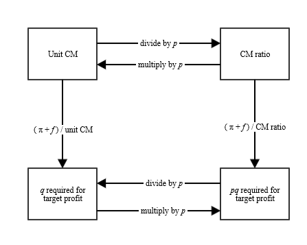
When I was an undergraduate student, I preferred unit CM. I would solve all class problems using unit CM. If I needed to solve for sales dollars required, I would just multiply the answer by p.
In many
3.3.4 Breakeven Analysis
A special case of the above analysis involves setting the target profit at zero. This is called breakeven analysis or breakeven point analysis.
It would be fair for a student to ask, then, “Professor Knox, if managers want to maximize profit, why would they care about the volume required to reach a π of zero?”
Good question, student. Your brownie points are in the mail. It’s because the future is uncertain, and π < 0 is really bad. Like I said earlier, just covering fixed costs is important to maximizing profits over time because if the firm doesn’t cover fixed costs it’s likely to go out of business.
(Just ask the federal government. Oh wait…no, nevermind).
As a matter of calculation, breakeven literally uses the same analysis as above, just holding π at zero.

Breakeven numbers provide managers with a line in the sand.
Margin of safety: the firm’s current sales (in units or sales dollars) minus the sales required for breakeven (in units or sales dollars).
The margin of safety figure captures how many sales the firm can lose before it reaches the breakeven point.
3.4 Target Profit for Multi-product Firms
3.4.1 Equations for Multi-Product Firms
What if the firm sells more than one product? Actually that’s the norm. Single-product firms are rare. But multiple products wreak havoc on all our neat and tidy equations introduced in Sections 3.2 and 3.3. Multiple products means multiple p variables, multiple q variables, and multiple v variables. It gets very messy very quickly. Some firms just embrace it and live in the soup of a C(·) that is miles long.
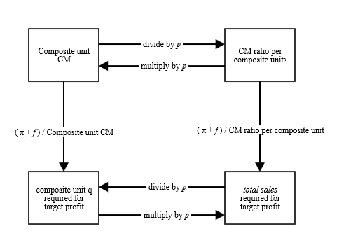
Luckily, there’s a shortcut that lets me use the same equations we discussed earlier for a multi-product firm. I just have to assume a certain sales mix of products and slightly change the equations’ wording.
$$\Large \frac{\pi + f}{Composite\ Unit\ CM} = Composite\ Unit\ q$$ $$\Large \frac{\pi + f}{CM\ Ratio\ per\ Composite\ Unit} = pq$$I’ve changed every mention of “q” or “units” to now be “composite unit q” or “composite units.” Composite units refers to a bundle of units of all the products a firm sells, at the expected sales mix. That is, a composite unit is a bundle of products that represents the sales mix.
Example 1
For example, let’s say a firm sells hand tools: hammers, nails, and saws. The expected sales mix is 2 hammers for every 5 boxes of nails and every 1 saw (or 2:5:1). A composite unit, then, is a bundle of eight items: 2 hammers, 5 boxes of nails, and 1 saw. I can solve this problem much like a single-product CVP problem if I temporarily act as if products are sold as this exact bundle of units.
If hammers have a unit CM of $5, boxes of nails have a unit CM of $1.50, and saws have a unit CM of $8, then the composite unit CM is $25.50
($5 * 2 hammers per composite unit + $1.5 * 5 boxes of nails per composite unit + $8 * 1 saw per composite unit).
If the firm has fixed costs of $1000 and the firm wants to reach a target profit of $1,040, I can calculate the number of composite units required to reach that target profit using the composite unit CM of $25.50. I need 80 composite units.
([$1,000 fixed costs + $1,040 target profit] / $25.50 composite unit CM = 80 composite units required to reach target profit.)
If I want to know how many hammers, specifically, must be sold to reach that target profit. I simply need to use the sales mix to convert from composite units to hammer units. In this case, the number of hammers sold at target profit is 160, since the sales mix is 2 hammers : 5 boxes of nails : 1 saw.
(80 composite units at target profit * 2 hammers per composite unit = 160 hammers at target profit).
Notice that the figure below still suggests you can convert from unit CM to CM ratio numbers using p. This refers to a composite p, though, as in prices of individual products weighted together using the sales mix.
Example 2
If the price of a hammer is $10, the price of a box of nails is $2 and the price of a saw is $20, then the price for a composite unit is as follows.
$10 per hammer * 2 hammers per composite unit = $20
$2 per box of nails * 5 boxes of nails per composite unit = $10
$20 per saw * 1 saw per composite unit = $20
20 + 10 + 20 = $50 price per composite unit.
I can convert from the number of composite units required to total sales required by multiplying by $50. If I need 80 composite units to reach target profit, then the total sales required to reach target profit is $4,000.
(80 composite units at target profit * $50 price per composite unit = $4,000 in sales at target profit).
Here’s a trick that uses the magic of the CM ratio. If you already know total revenue and total variable costs then you can calculate the CM ratio (i.e. the CM ratio per composite unit). You can calculate total sales required for target profit without ever defining the sales mix or calculating a composite unit.
Example 3
Assume a multi-product firm has total sales of $2,000,000, total variable costs of $1,200,000, fixed costs of $100,000. Next year’s target profit is $400,000 and the sales mix and cost structure (i.e. fixed costs and CM ratio) are expected to stay the same.
I need to determine how many sales dollars are required to reach next year’s target profit. First, I find the CM ratio: 0.4 or 40%.
([$2,000,000 total sales – $1,200,000 variable costs] / 2,000,000 total sales = 0.4 CM ratio)
Now, do I need to know the sales mix? Actually I don’t need to know it. The firm’s current sales mix is already reflected in the total sales and variable cost numbers. The CM ratio of 40%, then, already accounts for whatever sales mix they have. As long as the mix is expected to stay the same next period, I can ignore the details of it! The firm needs $1.25 million in total sales to reach target profit.
([100,000 fixed costs + $400,000 target profit] / 40% CM ratio = $1,250,000 total sales required to reach target profit)
All of these analyses are made simpler by assuming a predetermined sales mix. In actual practice the firm would want to test several different sales mixes as a form of sensitivity analysis. What if the firm sells more of product 1 and less of product 2 this month? What if the firm sells almost entirely product 3 next month? And so forth.
3.5 Cost Structure and Degree of Operating Leverage
CM ratio tells you the percentage of sales that is left over after accounting for variable costs. That is, it answers the question of how big total contribution margin is relative to total sales. Degree of operating leverage, or DOL, is similar but expresses the relationship between total contribution margin and profit, πf.
$$\Large DOL = \frac{Total\ CM}{Total\ CM\ – f} = \frac{Total\ CM}{\pi}$$If it helps you remember the DOL and CM ratio equations, just think of total contribution margin as the king or queen of the CVP kingdom: it is in the numerator atop both ratios.
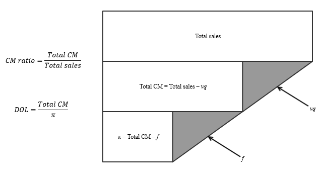
DOL tells you how many dollars of total CM it takes to earn one dollar of π. A high DOL suggest high fixed costs. Usually firms trade off between fixed costs and variable costs. If a firm invests in a large fixed cost piece of machinery, it usually is so it can save in variable costs from renting that machinery or buying machinery output from a supplier. This is a lot like renting versus owning a home. It is also part of the fundamental dilemma behind make-or-buy decisions from Chapter 2. Therefore if a firm has a high CM ratio, it is likely to have a high DOL. If the firm has a low CM ratio, it is likely to have a low DOL.
DOL and CM ratio capture something about firms’ confidence in customer value from their products. If a firm has a “sure winner” product and managers think sustained or growing customer value will keep sales steady or growing for the foreseeable the future, then they often try to lock in some of that customer value with fixed costs, which can create economies for scale for the firm. Long-term debt, long-lived assets, contracts with long time horizons, and so forth. These tend to increase fixed costs and decrease variable cost per unit, which in turn makes CM ratio and DOL both higher.
Of course high fixed costs are a problem if management is wrong and sales dip.
If a firm worries that customer value from its products will decrease or if there is some immediate threat to customer value, the firm is less likely to take on extra fixed costs. They still want to be in business if there is a dip in sales.
In short, the high DOL/high CM ratio path means bigger upside when scaling up but bigger exposure to risk from sales dips. The low DOL/low CM ratio path reduces exposure to risks from sales dips but also less profitability from scaling up.
You can tell a lot about a firm’s outlook from its DOL and CM ratio.
3.6 Special Orders and CVP analysis
Special orders, finally. Managers often have to make special order decisions without a settled price. The price is still up for negotiation. It’s important to know where your minimum acceptable price is, i.e. the price floor, in these circumstances. I’ll call these variable-price special order decisions.
There are four main varieties of variable-price special order decisions. They differ based on, first, whether the special order requires extra fixed costs to complete (such as special equipment or special licenses), and second, whether the firm has enough unused capacity to fill the special order.
Types of variable-price special order decisions
- No additional fixed costs and plenty of capacity
- No additional fixed costs and limited capacity
- Yes additional fixed costs and plenty of capacity
- Yes additional fixed costs and limited capacity.
It is important to understand total contribution margin, fixed costs, and variable costs before discussing variable-price special order decisions. All four variations of this decision are easily solved using contribution margin and cost-volume-profit principles. Here is the total CM equation.
$$\Large \pi+f= (p-v)q$$The floor is usually going to be the breakeven point, where π equals zero (if it’s important to the firm to consider cost of capital, you can include the cost of capital as a fixed cost). So it looks like this.
$$\Large f=(p-v)q$$As long as the firm requesting the special order is already certain of how many units it wants (which it usually is), you can simply solve for p from this equation.
$$\Large p=\frac{f}{q}+v$$Also remember I already set π equal to zero, so solving for p gives me the minimum price in the negotiations. The firm should be indifferent to a special order at this price and should accept anything above this price (ignoring strategic cost analysis for now). The f in this equation refers to fixed costs required for the special order, e.g. special licenses, special equipment, etc. This way, the special order price will at least cover those additional fixed costs, if they exist.
But how would one use this analysis to account for limited capacity? Limited capacity is mentioned in two of the four variations I listed above. Limited capacity means the firm only has capacity to produce a certain number of product units, and the special order would put the firm over that number. Accepting the special order, then, involves kicking out at least some regular paying customers.
It’s actually pretty simple: include the opportunity cost of kicking out
3.7 Constrained Resource Decisions
Chapter 1 introduces the basic equation of π. I argue that cost accounting information is information that helps the firm maximize π. In Chapter 2, I explored a few traditional scenarios where firms maximize π by choosing between discrete alternatives that have different π outcomes.
In Chapter 3, so far, I’ve discussed decisions where π is held constant, and the focus is on other variables in the profit equation. Sometimes the manager wants to know q, given a π of zero (i.e. breakeven decisions) or given a π of more than zero (i.e. target profit decisions). For variable-price special order decisions, the firm wants to know the minimum p when q and all other variables are held constant.
One additional type of decision follows this general pattern: constrained resource decisions. This decision arises in the following scenario.
- The firm sells multiple product lines.
- The firm can estimate the overall demand, q, for each product line (let’s assume there’s limited demand).
- The firm’s capacity of a key resource is insufficient to fill all demand in all the firm’s product lines.
The key resource in the third condition is the “constrained resource” that gives this type of decision its name. It can be a machine or employee with only so many hours to provide in a given period. It can be a limited material input. It can be a limited license or supplier. It can be limited by union contract. It can be a regulatory limitation, such as an emissions cap or a maximum number of driver hours allowed in a given period.
(Constraints affect firms decisions in many ways. My treatment of this decision barely scratches the surface. I discuss constraints further in Chapter 8.)
To make these decisions the manager has to prioritize its product lines in a way maximizes π. Should it produce all of product 1 first, and then use whatever constrained resource capacity is left to produce product 2? Or should it start by filling all product 2 demand, and then use leftover capacity to fill a part of product 1’s demand?
This decision is simpler than you might think. First, the decision is basically the manager ranking each product lines by its contribution margin and then filling each product line’s demand in that order. (These tend to be shorter-term decisions, and fixed costs don’t differ between alternatives. Thus the manager can look at contribution margin instead of overall profit.)
But because there’s a constrained resource, you cannot just compare raw contribution margin. Not all contribution margin dollars are equal because they use up the constrained resource’s capacity differently.
As an example, let’s assume product 1 has a unit CM of $100, and product 2 has a unit CM of $50. Seems pretty easy: fill product 1’s demand first, then use any leftover constrained resource capacity to fill part of product 2’s demand.
But now let’s also assume each unit of product 1 uses 10 hours on the constrained resource and each unit product 2 uses 2 hours on the constrained resource. Even though each unit of product 1 contributes twice as much as each unit of product 2, the firm can produce 5 times more product 2 units with its limited capacity of the constrained resource. The priority should actually be product 2 first and then product 1.
Put more formally the manager needs to know contribution margin per unit of the constrained resource. The manager needs to know how many units of the constrained resource each dollar of contribution margin costs.
$$\Large Constrained\ Unit\ CM= \frac{Unit\ CM}{Constraint\ Used\ per\ Unit}$$Consider this example with three product lines. (Notice the first row gives the units of the constrained resource available.)
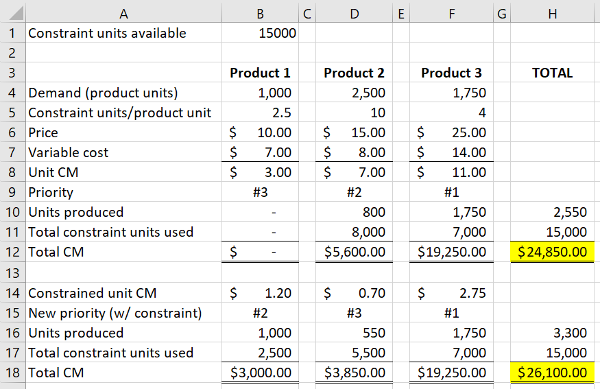
First I rank the priority of these product lines based on standard unit CM (see row 9). In order of priority, I produce as many of that product line I can until demand or the constraint is exhausted (see row 12).
Then, in contrast, I rank product lines based on their constrained unit CMs (see row 15). And then, in the new order or priority, I produce as many of each product line as possible until demand or the constraint is exhausted (see row 18).
Compare cells H12 and H18. Factoring in the constrained resources leads to a higher total contribution margin! That’s because we’re minimizing the units of constrained resource being traded off per dollar of contribution margin.
3.8 Final Note
I want to point out how everything in this chapter—total CM, unit CM, CM ratio, multi-product CVP, DOL considerations, variable-price special order decisions, and constrained resource decisions—flow naturally from separating C(·) into fixed and variable costs. These are not magic potions that some managerial accounting professor cooked up in a lab. “Let’s see if they can memorize this equation for the test! Mwahahaha!”
Instead they are the natural consequences of managers in practice seeking more information about their firm’s cost function, all in the interest of maximizing the firm’s profit. Once managers have made the assumptions that go along with fixed and variable costs, they have implicitly activated CVP analysis as an agent of profit maximization for their firm.
Isn’t that so cool! I’m still geeking out about it!